Topics (384k) Articles (398k) Users (410) Discussions (242) Comments (383) Files (13k) New article
For a quasihydrostatic bubbly mixture with gas void fraction , volume averaging gives the displayed mass density. A body displacing mixture volume has approximate buoyant force . A floating body of mass therefore needs ; gas release can increase its draft until the required displacement exceeds its available watertight volume. This mechanism explains a possible loss of flotation without making sinking inevitable in every gas plume. Upward liquid flow, turbulence and nonuniform bubble distributions require additional hydrodynamic forces beyond this simple mixture model.
The centre of buoyancy is the point through which the resultant hydrostatic buoyant force acts. In a uniform fluid under uniform gravitational acceleration, it is the volume centroid of the displaced fluid. For a floating body its position generally changes when the body tilts, because the displaced volume changes shape.
A bubble chamber using liquid hydrogen as both target and recording medium. For a beam interaction on a proton, the target's initial momentum can usually be approximated as zero on the scale of the beam momentum. This makes four-momentum conservation especially useful: the initial state does not include the unknown motion of a proton bound inside a heavier atomic nucleus. The approximation still neglects molecular binding and thermal motion.
Stereoscopy enables three-dimensional track reconstruction.[ref]
How It Works: Bubble Chamber (CERN teaching archive). How it works, views
Calibrated camera positions and optical geometry are needed before a photographed arc becomes a physical radius of curvature. Neutral particles do not directly leave the same continuous ionization trail as charged particles; an interaction or decay can instead reveal them through charged secondary tracks. A photon's inferred path between interactions is not a photographed luminous line.In a uniform magnetic field, with negligible stopping power and elastic scattering over the fitted segment, the transverse projection is a circle. The Lorentz force turns transverse momentum at angular rate , givingHere is measured in the plane perpendicular to the magnetic field. The relation remains valid with relativistic physical momentum; it does not require . Thus curvature determines magnetic rigidity, not mass or kinetic energy alone. For chosen , and , . This is an invented example, not a fit to a historical photograph. Reconstructing a three-dimensional helix also determines the component parallel to the magnetic field; the transverse radius of curvature alone does not. Determining the sign of electric charge additionally requires the field direction and the direction of travel, as in the charge-sign ambiguity of a curved track.
Why can hot liquid wait for a charged particle rather than immediately turn into vapor? A small cavity costs surface energy. Consider an original macroscopic capillarity model at fixed temperature with surface tension , imposed liquid pressure , and driving difference , where is the planar-interface vapor pressure. Neglect dissolved gas, interface thickness, heat transfer and curvature dependence of . The reversible formation-work approximation isThe first term charges for surface area; the second rewards the new vapor volume. This is a macroscopic free energy model, not the energy that an actual detector must receive as localized heat. It shares the capillarity balance used in the cloud-chamber expansion model, but the new phase is now a bubble.
Differentiating givesAt the critical nucleus, . The barrier is a maximum: cavities smaller than tend to shrink, while larger ones can grow in this model. Doubling halves and quarters if stays fixed. This explains the strong sensitivity to operating conditions without claiming a universal detector threshold.
Choose and solely for a teaching example. ThenFor the same chosen and twice the driving pressure, and . These are calculated formation-work scales, not measured bubble thresholds for diethyl ether or any other substance.
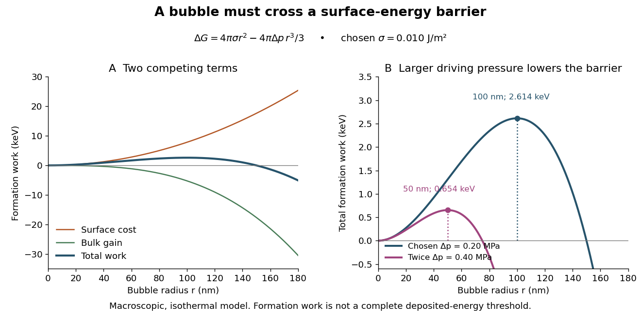
A simplified way to discuss localization is to stipulate deposited energy within a segment of length and a trial conversion fraction . A toy criterion gives an energy per unit length scale . It is only a bookkeeping estimate: a real bubble also needs latent heat, must exchange heat, and is affected by the spatial pattern and time scale of energy deposition. Consequently neither a single stopping power value nor this barrier alone predicts detection efficiency or the number of bubbles. Two tracks with the same mean stopping power can distribute their energy differently on the scale of a critical nucleus.
Unlike the Blackett-Occhialini triggered cloud-chamber experiment, Glaser used counter-controlled flashes after expansion. A detector trigger can select recording in sensitive liquid; subsequent expansion cannot recover a vanished latent track.[ref]
Elementary Particles and Bubble Chambers by Donald Arthur Glaser. pp. 537, 541, 550: timing distinction
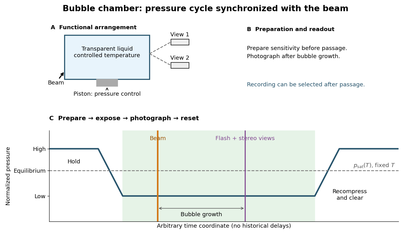
Bubble-chamber pressure cycle and photographic readout
. Original functional diagram with an arbitrary time coordinate and chosen normalized pressure levels. The dashed equilibrium line assumes fixed temperature; no measured waveform, apparatus scale or historical delay is reproduced. Details.The diagram deliberately separates the preparation through thermodynamics from the readout decision. Its green interval is a stipulated operating window, not a prediction from pressure alone. Excess superheating can increase unwanted nucleation; insufficient superheating can suppress tracks. A useful proposed sensitivity check holds the readout settings fixed while varying pressure or temperature, with matched background exposures. A proposed timing check moves the beam within the cycle; a proposed optical check varies flash delay to distinguish growing bubbles from changes in spatial resolution. These are experimental design examples, not additional historical measurements.
Donald Arthur Glaser developed the bubble chamber in 1952 during experimental particle research at Michigan.[ref]
His 1960 lecture, Elementary particles and bubble chambers, describes evacuated capillary bulbs containing pure diethyl ether. Cooling one bulb reduced pressure; the other remained hot. A cobalt-60 source initiated boiling. Small glass chambers subsequently used hot-oil baths, hand-cranked pistons and high-speed photography. Automatic cycling with counter-controlled flashes produced finer tracks. Local ionization deposits energy that can initiate bubble nucleation.[ref]
Later metal-chamber photographs compared operation with and without a nearby radioactive source: wall boiling occurred without interior tracks; irradiation produced tracks before disruptive flow ended sensitivity.[ref]
Elementary Particles and Bubble Chambers by Donald Arthur Glaser. pp. 539–543, Fig. 6
These observations separate two questions: can radiation start boiling, and can a detector preserve the geometry of a passing charged particle? Whole-vessel boiling alone answers only the first. Wall background, finite sensitivity and growth before photography constrain the second.
A bubble-chamber track is a line of growing vapor bubbles seeded by ionization along a charged particle path in a superheated liquid. The bubbles scatter illumination and can be photographed from multiple directions to reconstruct the path in three dimensions.
In a known magnetic field, curvature constrains the particle's momentum and the sign of its electric charge; increasing ionization toward a stopping point can add information about energy loss. Bubble size and photographic blur set the visible trail width, so that width is not the particle's physical diameter. Neutral particles can remain invisible until an interaction produces charged secondaries.
For an entire function , let with noninteger real , and choose the branch of the complex logarithm with . On the cut ray , the bank whose argument approaches has value , while the other bank has argument approaching and value . The signed jump is therefore when defined as . Stating the branch and order of subtraction removes the sign ambiguity. A keyhole contour uses this phase relation to convert its two bank integrals into a constant multiple of one real or radial integral.
The effective electric charge associated with electric polarization is bound charge. For polarization density , its volume charge density is . At a boundary with unpolarized surroundings, its surface charge density is , where is the outward unit normal vector.
For a real shell potential , define and , with value one at zero. Angular integration of its three-dimensional Fourier transform gives , where the momentum transfer has wave-number magnitude . Substitution in the first Born approximation proves the displayed scattering amplitude. It is real. Its squared modulus is a nonzero order- differential scattering cross-section, whose optical theorem counterpart requires the order- imaginary part of the forward amplitude from the next Born term. Thus squaring the first-order amplitude does not supply a consistently unitary second-order amplitude.
For , with real and , the first Born approximation gives the scattering amplitudeIndeed, orienting the polar axis along the momentum transfer gives the angular integral , and the remaining integral is . The differential scattering cross-section is .
The limit at fixed nonzero produces the Rutherford differential cross-section for a Coulomb potential. The unscreened interaction has long range, so this limiting calculation by itself does not establish the validity of a naive Born approximation to the full Rutherford scattering state. The exact Rutherford scattering amplitude has an additional phase, while its modulus agrees with the Rutherford differential cross-section.
In On the Constitution of Atoms and Molecules, Part I (1913), pp. 8–9, Niels Bohr interprets existing hydrogen discharge and astronomical spectra. Electrical discharge in a vacuum tube removes electrons; recombination supplies spectral lines. This is a theoretical interpretation, without a reported spectrograph of his own.[ref]
On the Constitution of Atoms and Molecules, Part I by Niels Bohr. Part I, section 2, pp. 8–9: existing spectra
An actual optical obstacle appears in Theodore Lyman's measurements: hydrogen discharge light entered an evacuated spectrograph directly through a slit, avoiding a transmitting window. A concave reflection diffraction grating dispersed the light onto photographic film. Pumping preserved the vacuum; a second slit supplied a known spectral displacement for wavelength calibration. Gas contamination and vacuum leaks limited the measurement. This apparatus resolved ultraviolet spectral lines; it did not image orbits.[ref]
Theodore Lyman, Pioneer of Ultraviolet Vacuum Spectroscopy by Paul Horowitz. Paul Horowitz, Theodore Lyman, Pioneer of Ultraviolet Vacuum Spectroscopy, pp. 3–4, figures 2–5: windowless discharge connection, grating, film, pumping and dual-slit calibration
For a separate original calibration exercise, suppose an idealized spectrograph returns synthetic vacuum line positions for , with chosen additive offset . Assume its dispersion scale is already known and only this offset is uncertain. Compare the finite-mass prediction with the fixed-nucleus prediction . Calibrate each model using only the line: . Then hold that offset fixed and test the other lines with residualsFor the finite-mass model every . The fixed-nucleus model has and residuals , , . Algebraically : one additive calibration cannot absorb a multiplicative change of the wavelengths. Allowing an unknown multiplicative dispersion factor as well would make the two models degenerate in this exercise, so independent scale calibration matters.
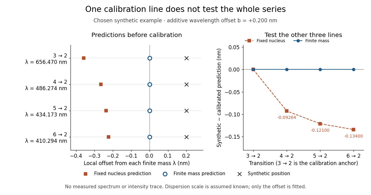
Balmer series predictions tested after calibrating one line
. Original synthetic calibration exercise with chosen . Left: finite-mass vacuum predictions and deliberately offset synthetic positions, displayed on a separate local wavelength axis for each line. Right: model residuals after anchoring the line; the remaining three lines test the prediction. Symbols are exact synthetic inputs and calculated results, not historical observations, error bars or an intensity trace. Details. Hydrogen transition wavelengths in the Bohr model by  Codex 0 Created 2026-10-18 Updated 2026-10-20
For emission take integers . Applying conservation of energy to the model's internal energy difference, while neglecting the much smaller whole-atom photon recoil, givesThus Johannes Robert Rydberg's Rydberg formula is a difference of two energy levels expressed as a spectroscopic wavenumber. The same constants determine every line; there is no new parameter for each electronic transition. With the chosen inputs, . All wavelengths below are calculated in vacuum, not air, and are rounded model predictions rather than historical measurements.
The conventional names commemorate Theodore Lyman and Johann Jakob Balmer. Fixing produces the ultraviolet Lyman series, beginning with the Lyman-alpha line; fixing produces the Balmer series. As , the wavelength approaches : at the Lyman limit and for the Balmer series. Crowding follows directly from . Discreteness therefore coexists with a series limit.
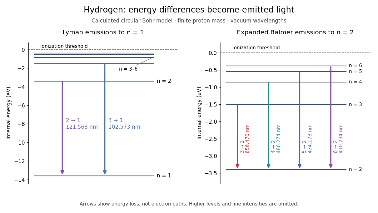
Correct line positions do not give wave intensities, lifetimes or electric-dipole selection rules for hydrogen. Those require a theory of the wavefunctions and their coupling to electromagnetic radiation. The circular model also omits spin, relativistic corrections and the Lamb shift. Its successful gross energy levels do not make its assumed orbits modern atomic orbitals.
Pinned article: Introduction to the OurBigBook Project
Welcome to the OurBigBook Project! Our goal is to create the perfect publishing platform for STEM subjects, and get university-level students to write the best free STEM tutorials ever.
Everyone is welcome to create an account and play with the site: ourbigbook.com/go/register. We belive that students themselves can write amazing tutorials, but teachers are welcome too. You can write about anything you want, it doesn't have to be STEM or even educational. Silly test content is very welcome and you won't be penalized in any way. Just keep it legal!
Intro to OurBigBook
. Source. We have two killer features:
- topics: topics group articles by different users with the same title, e.g. here is the topic for the "Fundamental Theorem of Calculus" ourbigbook.com/go/topic/fundamental-theorem-of-calculusArticles of different users are sorted by upvote within each article page. This feature is a bit like:
- a Wikipedia where each user can have their own version of each article
- a Q&A website like Stack Overflow, where multiple people can give their views on a given topic, and the best ones are sorted by upvote. Except you don't need to wait for someone to ask first, and any topic goes, no matter how narrow or broad
This feature makes it possible for readers to find better explanations of any topic created by other writers. And it allows writers to create an explanation in a place that readers might actually find it.
Figure 1. Screenshot of the "Derivative" topic page. View it live at: ourbigbook.com/go/topic/derivativeVideo 2. OurBigBook Web topics demo. Source. - local editing: you can store all your personal knowledge base content locally in a plaintext markup format that can be edited locally and published either:This way you can be sure that even if OurBigBook.com were to go down one day (which we have no plans to do as it is quite cheap to host!), your content will still be perfectly readable as a static site.
- to OurBigBook.com to get awesome multi-user features like topics and likes
- as HTML files to a static website, which you can host yourself for free on many external providers like GitHub Pages, and remain in full control

Figure 2. You can publish local OurBigBook lightweight markup files to either OurBigBook.com or as a static website.
Figure 3. Visual Studio Code extension installation.
Figure 5. . You can also edit articles on the Web editor without installing anything locally. Video 3. Edit locally and publish demo. Source. This shows editing OurBigBook Markup and publishing it using the Visual Studio Code extension. 
- Infinitely deep tables of contents:




All our software is open source and hosted at: github.com/ourbigbook/ourbigbook
Further documentation can be found at: docs.ourbigbook.com
Feel free to reach our to us for any help or suggestions: docs.ourbigbook.com/#contact