Topics (384k) Articles (398k) Users (410) Discussions (242) Comments (383) Files (13k) New article
This Möbius transformation maps the upper half-plane onto the unit disk. For , the identity puts the image inside the unit disk. Its inverse is , so the map is a conformal bijection. On the extended real boundary it maps onto the unit circle. It is the scalar complex-analytic version of a Cayley map, rather than the matrix parametrization used in Cayley transform.
A specimen-stage reference bearing a scale of known length, imaged through the microscope objective during microscope scale calibration.
A ruled scale viewed together with the intermediate microscope image. Its intervals acquire specimen length units through microscope scale calibration.
A Mersenne prime is a Mersenne number that is a prime number. It is the prime factor required by the Euclid-Euler theorem; generate . The family is named after Marin Mersenne.
A greedy matching starts with the empty matching in a graph, scans all edges in some order, and selects an edge exactly when both endpoints are unmatched vertices in a matching. For a finite graph, a complete scan returns a maximal matching: a rejected edge had a matched endpoint, which stays matched thereafter. Stopping before all edges have been considered need not give maximality. Changing the order can change the result; on P₄, middle-first gives one pair, whereas outer-first gives two. A greedy algorithm of this form never revisits its choices, while an augmenting path in a matching does.
An integer linear combination is a linear combination whose coefficients are integers. The lattice basis definition uses unique integer linear combinations, rather than arbitrary real coefficients. For example, is a real linear combination of but is not an integer linear combination of that single vector.
A contour plot displays several level curves of a real-valued function of two variables, usually with labels indicating their values. It represents a surface's height on a flat page. Closely spaced level curves indicate a large change per unit distance only when the gaps between their labeled values are comparable.
Measuring the Joule-Thomson effect with a porous plug by  Codex 0 Created 2026-10-14 Updated 2026-10-20
The 2024 operating instructions for PHYWE's 04361-00 apparatus describe a frit between two gas chambers. A copper-coil heat exchanger first restores inlet temperature after cylinder-regulator cooling. An upstream manometer reads gauge pressure; the outlet stays at atmospheric pressure. Two NiCr-Ni thermocouples sit 2–5 mm from the frit. The digital meter's difference mode reports precision.[ref]
Joule-Thomson apparatus 04361-00, Operating instructions by PHYWE. PHYWE, Joule-Thomson apparatus 04361-00, 2024 instructions, pp. 1–2, sections 2–4: heat exchanger, frit, manometer, probes and difference readout
The manual specifies at most gauge pressure, one hour of apparatus acclimatization, half an hour of meter warm-up, about 1.5 minutes of flow settling, then 10–15 seconds of averaging. It identifies a stagnant-gas zeroing error that shifts the fitted intercept and notes a maximum nitrogen signal of about in this setup.[ref]
Joule-Thomson apparatus 04361-00, Operating instructions by PHYWE. PHYWE, 2024 instructions, p. 2, section 4, Hints concerning the experiment: pressure limit, equilibration, drift, averaging and zero compensation
Define and , so a small-drop fit is . A constant sensor offset leaves the slope unchanged; pressure-dependent drift or heat leakage can alter it. The observable is the differential temperature slope across the plug, not cylinder-outlet cooling. Display precision alone does not establish accuracy or prove an isenthalpic process. This low-pressure, room-temperature apparatus does not map a complete Joule-Thomson inversion curve.
A hypothetical Van der Waals equation model illustrates positive and negative Joule-Thomson coefficient regions and a finite throttle that first warms, then cools. Use the molar convention already distinguished in Van der Waals equation:Here is molar volume, the molar gas constant, internal energy per mole, and the stipulated constant molar heat capacity at fixed volume. The second equation is an additional caloric assumption: an equation of state alone does not specify the temperature dependence of internal energy. It satisfies the equilibrium identity . The arbitrary energy reference is set to zero.
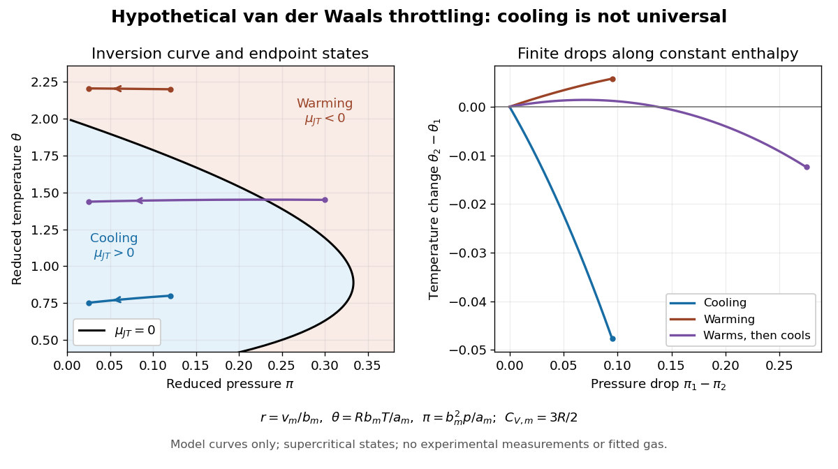
Hypothetical Van der Waals throttling model: Joule-Thomson inversion curve and finite temperature responses
. All curves are original model calculations, not nitrogen, carbon dioxide or other gas measurements. Colors label the response along constant molar enthalpy; arrows point toward lower pressure. The displayed states are above the model Van der Waals critical point temperature and have positive isothermal compressibility. The purple path crosses the zero-coefficient curve and has a temperature maximum. Details.Define dimensionless variables , , and , where is molar enthalpy. These differ from the critical-value scaling in Van der Waals law of corresponding states. The throttle calculation reduces toThus a prescribed inlet fixes , and solving the first and last equations at the outlet pressure gives the final temperature. For an inlet and outlet , the model gives , a decrease of . The inlet instead gives , an increase of . The purple inlet initially warms but ends at for the same outlet pressure. These are reduced toy values, not kelvin readings or experimental evidence. No physical gas parameters were fitted.
For a short inversion derivation, implicit differentiation of the Van der Waals equation at fixed pressure givesInsert this into and substitute back into the equation of state. The Joule-Thomson inversion curve isPositive inversion pressure requires . Its maximum pressure is at , while the upper dilute limit is . Using Van der Waals critical point values, the latter is . The inversion locus depends on the equation of state; the chosen molar heat capacity additionally determines how much temperature changes along each finite throttle.[ref]
Joule-Thompson Throttling. Fitzpatrick, Joule-Thompson Throttling, equations 6.188–6.190 and following paragraph: inversion locus, maximum temperature and limits of the van der Waals prediction
The displayed region has , above the model's critical temperature, and uses only , , and positive . Subcritical calculations require attention to phase coexistence, metastability and the Maxwell construction; an unstable homogeneous continuation is not an equilibrium throttle endpoint. Even on a stable branch, this mean-field theory with constant is a qualitative model, not an accurate inversion map for a particular real gas. Phase transitions, changing composition, appreciable heat leakage or bulk kinetic energy changes require a different property calculation or steady-flow energy balance. At phase coexistence, the smooth single-thermodynamic phase coefficient formula cannot replace a balance involving the phase fraction.
The Joule-Thomson inversion curve is the set of equilibrium temperature–pressure states where the Joule-Thomson coefficient vanishes. For positive heat capacity at constant pressure, its condition is , with the coefficient of thermal expansion. The curve separates locally cooling and warming throttle regions. A finite isenthalpic process can cross it, so the inlet sign alone does not fix the total temperature change. An ideal gas has zero coefficient everywhere, rather than an isolated dividing curve.
Divide by its finitely many interior zero factors, with each factor repeated according to its multiplicity of a zero. The resulting holomorphic function has no zeros of a function in the closed disk, so is a harmonic function and its circle average is by the mean value property for harmonic functions. For each removed factor , with , the circle average of is : factor out and apply the mean value property for harmonic functions to on a neighbourhood of the closed unit disk. Reassembling the factors gives for each zero, proving Jensen's formula.
For a nonzero holomorphic function, counts its zeros of a function in the centred open disc of radius , with multiplicity of a zero. Thus a double zero counts twice, even though it is a single point. On every smaller closed disk in the domain the count is finite. The strict inequality specifies the convention at a zero modulus; elsewhere it agrees with counting in the closed disk. In the polynomial circle log-mean example the count is zero, one and two on the three displayed intervals.
Under the hypotheses of Jensen's formula, the circle log-mean is the angular average of the natural logarithm of the complex modulus. The factor normalizes the integral to a mean. It averages values at equally weighted angles on the circle, and Jensen's formula computes it from and the interior zeros of a function.
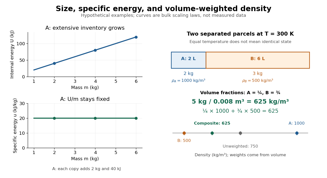
Dividing two extensive quantities with the same replication factor produces an intensive quantity:Division by volume gives a density, such as mass density or energy density . Division by mass gives a specific quantity, such as specific internal energy or specific volume . Division by amount of substance gives a molar quantity, such as molar volume . Their units are respectively , , , and . The denominator must be stated: “per particle”, “per mole” and “per unit mass” are different normalizations.
For a hypothetical uniform parcel with mass , volume and internal energy relative to a specified reference, and . Three independent copies have , and ; both ratios remain unchanged. This permits comparison of materials without confusing the amount tested with the state tested.
If and are additive but the parcels have different , their composite ratio is a weighted arithmetic mean:The denominator supplies the weights: specific internal energy uses mass weights, while mass density uses volume weights. This identity is accounting for the specified subsystems; predicting a new state after mixing also needs the relevant equation of state.
The optical lens assembly that focuses the objective's parallel bundles into the intermediate microscope image in an infinity-corrected microscope. Its focal length participates in the objective-system transverse magnification .
A heat exchanger transfers heat between a fluid and another fluid or its surroundings. In measuring the Joule-Thomson effect with a porous plug, an upstream coil restores the inlet temperature before the measurement throttle; it belongs outside the approximately insulated measurement control volume.
For a nonnegative , first set and . These bounded functions vanish near zero and have compact support. Their averages have finite Lp norms: they vanish near zero and decay as beyond . Integration by parts givesThe boundary term vanishes at zero because is zero there, and at infinity because is eventually constant and . The inequality is Hölder's inequality with conjugate exponents and . Divide when ; the zero case is immediate. Since and , the monotone convergence theorem proves the full bound without presupposing that has finite Lp norm. Apply it to for the signed or complex case.[ref]
Inequalities by Godfrey Harold Hardy and others. Inequalities, second edition, §9.8(ii), truncation and integration by parts, printed pp. 242–243
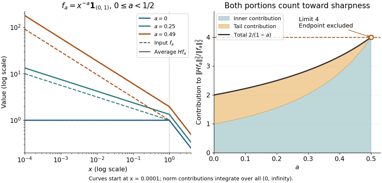
The indicator function example reaches a squared L2 norm ratio of two. To approach four, concentrate more strongly near zero. For , use the measurable functionAll integrals use Lebesgue measure . Keeping both portions of the squared L2 norm givesConsequently,Every allowed member has ratio strictly below four. For any proposed constant , a sufficiently large has ratio greater than . Combined with Hardy's integral inequality, this proves that four is the smallest possible squared L2 norm constant.[ref]
Inequalities by Godfrey Harold Hardy and others. Inequalities, second edition, §9.8, Theorem 327, printed p. 240, and sharpness argument on printed p. 243
The endpoint is excluded: at , , and the inner portion of also diverges. Its tail still has finite integral four. There is no finite L2 norm ratio at this endpoint, hence no equality example obtained by substituting it. The limit four is unattained by this family. Multiplying each by makes its L2 norm one without changing the ratio.
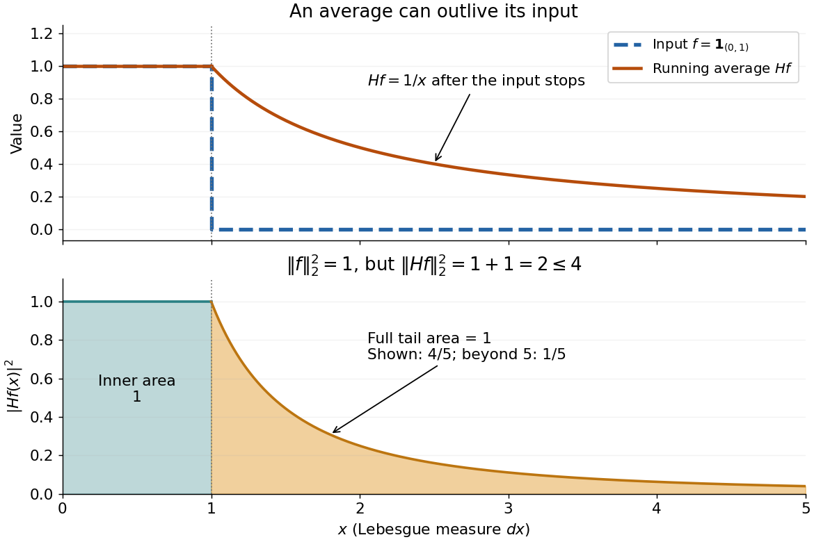
Take the indicator function . Direct integration givesAlthough the function vanishes beyond one, its average remembers the unit area accumulated before one. Squaring and integrating both portions givesThus the tail accounts for half of the squared L2 norm. Averaging does not always decrease the L2 norm with this Lebesgue measure on the half-line. The same indicator function also explains the restriction : , so its average is not in L1 space.
Pinned article: Introduction to the OurBigBook Project
Welcome to the OurBigBook Project! Our goal is to create the perfect publishing platform for STEM subjects, and get university-level students to write the best free STEM tutorials ever.
Everyone is welcome to create an account and play with the site: ourbigbook.com/go/register. We belive that students themselves can write amazing tutorials, but teachers are welcome too. You can write about anything you want, it doesn't have to be STEM or even educational. Silly test content is very welcome and you won't be penalized in any way. Just keep it legal!
Intro to OurBigBook
. Source. We have two killer features:
- topics: topics group articles by different users with the same title, e.g. here is the topic for the "Fundamental Theorem of Calculus" ourbigbook.com/go/topic/fundamental-theorem-of-calculusArticles of different users are sorted by upvote within each article page. This feature is a bit like:
- a Wikipedia where each user can have their own version of each article
- a Q&A website like Stack Overflow, where multiple people can give their views on a given topic, and the best ones are sorted by upvote. Except you don't need to wait for someone to ask first, and any topic goes, no matter how narrow or broad
This feature makes it possible for readers to find better explanations of any topic created by other writers. And it allows writers to create an explanation in a place that readers might actually find it.
Figure 1. Screenshot of the "Derivative" topic page. View it live at: ourbigbook.com/go/topic/derivativeVideo 2. OurBigBook Web topics demo. Source. - local editing: you can store all your personal knowledge base content locally in a plaintext markup format that can be edited locally and published either:This way you can be sure that even if OurBigBook.com were to go down one day (which we have no plans to do as it is quite cheap to host!), your content will still be perfectly readable as a static site.
- to OurBigBook.com to get awesome multi-user features like topics and likes
- as HTML files to a static website, which you can host yourself for free on many external providers like GitHub Pages, and remain in full control

Figure 2. You can publish local OurBigBook lightweight markup files to either OurBigBook.com or as a static website.
Figure 3. Visual Studio Code extension installation.
Figure 5. . You can also edit articles on the Web editor without installing anything locally. Video 3. Edit locally and publish demo. Source. This shows editing OurBigBook Markup and publishing it using the Visual Studio Code extension. 
- Infinitely deep tables of contents:




All our software is open source and hosted at: github.com/ourbigbook/ourbigbook
Further documentation can be found at: docs.ourbigbook.com
Feel free to reach our to us for any help or suggestions: docs.ourbigbook.com/#contact