Topics (384k) Articles (398k) Users (410) Discussions (242) Comments (383) Files (13k) New article

For sufficiency, take a matching in a graph of maximum size and suppose a left vertex is unmatched. Follow unused edges from left to right and matching edges back to the left. An unmatched reachable right vertex yields an augmenting path in a matching, contradicting maximal size. Otherwise let be the reachable left and right sets. Every member of is matched to a distinct member of , and every member of is reached this way. Since , we obtain , contradicting the Hall condition. Finiteness ensures that a maximum-size matching in a graph exists.
The alternative Hall induction through a tight set uses mathematical induction: a proper nonempty subset with splits off a balanced induced subgraph; without such a tight set, deleting one chosen edge's endpoints preserves the Hall condition on the smaller left side.
A system of distinct representatives for a finite indexed family of finite sets chooses one element per index, with all choices distinct. Form a bipartite graph with left vertex set , right vertex set , and edges whenever . Matching saturation of is precisely a system of distinct representatives. Hence Hall's marriage theorem says that such choices exist exactly when for every subset . Repeated equal sets still have separate indices and separate demands.
In a unit-capacity assignment problem, left vertices represent demands and right vertices represent individually usable resources; an edge records compatibility. All constraints must be encoded by those allowed pairs and by using each resource at most once. Hall's marriage theorem decides feasibility. Costs belong to an additional mathematical optimization problem; precedence between jobs or requirements for consecutive slots need additional modelling.
The authored Notes on the design of a conference scheduler by David R. MacIver (Implementation, 7 August 2022) illustrates a Hall obstruction with four talks confined to three slots. With one talk per slot, that subset has size four and a graph neighbourhood of size three. An unused slot outside its graph neighbourhood does not remove the bottleneck. In the three-job example above, the same scheduling model instead has two complete assignments.
The allocation exercise in Graph Theory by Reinhard Diestel (Matching, Covering and Packing, printed p. 20, Exercise 9) asks for disjoint subsets of prescribed nonnegative integer sizes . Replace demand by left vertices with allowed resource set . Hall's marriage theorem gives exactly the conditionFor a numerical instance, let , , and . The separate demands and their combined demand fit, and works. Raising to two leaves both individual tests valid but demands four distinct resources from a set union of size three. This is the same collective obstruction with repeated demand vertices.
The Hall condition requires enough distinct neighbours for every subset of the specified left vertex set in a finite bipartite graph. Checking the whole left set establishes only one inequality. Checking singleton sets establishes only that each left vertex has positive degree of a vertex. Overlapping lists can pass both tests and still fail to admit matching saturation of the left side.
In 2014, Gabriele Rosi and colleagues used atom interferometry: two rubidium-87 clouds prepared by laser cooling in vacuum, apart, received shared three-pulse Raman transitions spaced by . Fluorescence readout and paired-fringe ellipse fitting yielded differential wave phase. Twenty-four tungsten alloy cylinders, about total, moved between C and F. Cloud subtraction rejected shared vibration; configuration subtraction isolated the source change.[ref]
Precision Measurement of the Newtonian Gravitational Constant Using Cold Atoms by Gabriele Rosi and others. Main text pp. 3–5; Methods pp. 13–14; Fig. 1 caption p. 21
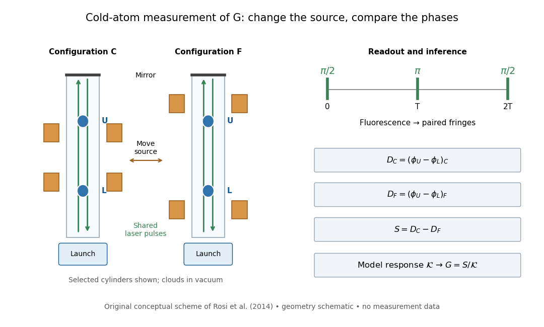
Precision Measurement of the Newtonian Gravitational Constant Using Cold Atoms by Gabriele Rosi and others. Main text pp. 3–5 and Fig. 1 caption p. 21
Details.Calibration used timed flight and light-sheet crossings; mirror tilt compensated Earth rotation. Wave vector reversal rejected unwanted shifts. Modeling included source Newtonian gravitational potential, atom trajectories, cloud distributions and moving supports. Source positioning, mass density variation and cloud geometry limited the reported combined relative standard uncertainty to parts per million.[ref]
Precision Measurement of the Newtonian Gravitational Constant Using Cold Atoms by Gabriele Rosi and others. Main text pp. 5–6; Methods pp. 14–18; Table 1, p. 27
To understand the subtraction without reproducing that full analysis, consider an ideal atom interferometer in uniform vertical acceleration during each pulse sequence. Let be its signed effective vertical wave vector component and the pulse spacing. Its acceleration-dependent wave phase is ; labels U and L denote upper and lower clouds. The double difference is thenA background field identical in C and F cancels even if it differs between the two clouds. In a fixed-geometry, linear-response model, write , where is calculated from the source mass density, calibrated pulse sequence and atom trajectories. Thus . Measuring wave phase accurately is one part of the task; calculating accurately is another. The real nonuniform field and finite clouds require the trajectory-dependent analysis described above rather than this uniform-field approximation.
A laboratory determination of the gravitational constant must connect a sensor's reading to a gravitational signal from independently characterized masses. For an ideal two-point mass force measurement, invert the model:These are signed small changes obtained by taking the logarithmic derivative, not an instruction to add standard uncertainties with signs. For independent small input uncertainties, linear propagation of uncertainty instead givesCorrelated inputs require their covariances too. In particular, common geometric calibration errors must not be treated as independent simply because several distances were recorded.
For a concrete model check, hold the actual force and masses fixed but overestimate a true by . The exact inferred ratio isThe resulting bias is parts per million, already comparable with the relative standard uncertainty of the recommended gravitational constant. A sensor can resolve very small changes while its inferred answer remains limited by source geometry. The example concerns one idealized separation; it is not an uncertainty estimate for any actual experiment.
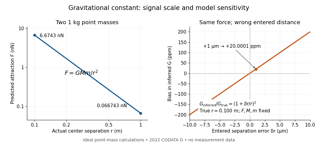
Weak laboratory attraction and the geometric sensitivity of an inferred gravitational constant
. Left: ideal force between two stipulated point masses using the 2022 recommended gravitational constant. Right: exact model bias when only the separation entered in the inference changes. These curves are calculations, not measurement data. Details.Making the source mass larger or bringing it closer strengthens the signal, but also makes detailed mass density and geometry important. Nearby apparatus supplies its own Newtonian gravitational field; electromagnetic shielding does not remove that attraction. Sensor offsets, changing temperature, vibration and source motion can imitate or alter a signal. The Cavendish experiment illustrates calibration of a torsion constant; a different sensor requires its own calibrated response and a full source model.
Repeating readings can reduce independent measurement noise, but a fixed scale error survives averaging. A useful experiment deliberately changes the source configuration, checks whether the signal follows the predicted change, and characterizes what moves with the source. A systematic error that changes with that configuration also survives background subtraction. Comparing methods with different sensors and different dominant errors is therefore valuable.
An orbit around an isolated source constrains its standard gravitational parameter rather than independently measuring the source's mass and the gravitational constant. In the test particle approximation, a circular orbit of radius and orbital period satisfiesThe left equation equates the required centripetal acceleration to the gravitational acceleration. More generally, a Kepler orbit depends on the same . In the exact relative two-body problem, replace by .
For any positive dimensionless number , replacing by and by leaves and every predicted test particle trajectory unchanged. This is the gravitational mass degeneracy: more observations of the same orbit can refine without separating its factors. A laboratory source whose mass is calibrated independently supplies the missing information.
Consequently an astronomical mass expressed in kilograms as inherits measurement uncertainty from , even if is known much more precisely. To first order,When the relative standard uncertainty of is negligible, that of is approximately . Conversely, the ratio of two source masses inferred using the same is , so this common factor cancels. That distinction explains how excellent orbit determination can coexist with less precise absolute astronomical masses.
A specified test for germination, recording the endpoint, conditions and observation window. For a proposed red/far-red light test, use randomization to allocate one seed lot to darkness, red, red then far-red, and red then far-red then red. Match hydration, temperature, handling and elapsed time before counting; use sham waiting periods to equalize schedules. Use dish replication, retain the dark scientific control, and record radicle emergence using an observation procedure that does not itself provide an uncontrolled light treatment. This is a proposed design, not a claim about the 1952 paper's randomization or replication.
As an original hypothetical counting example, begin with seeds in one dish. Suppose 12 first meet the radicle endpoint by 24 hours, eight additional seeds by 48 hours, and four additional seeds by 72 hours. These invented event counts giveand cumulative sample proportions , and . The 48-hour increment is , not ; the latter includes earlier events. Counting the same emerged radicle again at each inspection would inflate the total. These numbers illustrate bookkeeping, not biological rates or treatment effects.
With a fixed denominator and irreversible classification of the first endpoint event, the set counted at an earlier inspection is a subset of the set counted later. Hence and cannot decrease. This short proof applies to cumulative germination counts even if a later seedling dies. A count of currently surviving seedlings has a different definition and can decrease.
For treatment comparisons, the dish may be the experimental unit: seeds in the same dish share conditions. Forty seeds in one dish do not supply forty independent dish replicates. Report the sample size, replication, endpoint time and denominator; a sample proportion by a deadline measures this assay's outcome, not an unconditional fraction with seed viability.
The 1952 experiment used Grand Rapids lettuce seeds on wetted blotters in covered dishes. After 16 hours in darkness, seven lots of 200 received successive alternating exposures: one minute of red light at –, then four minutes above , with one lot removed after each exposure. Treated lots and a dark scientific control remained at for two days; germinated seeds were counted. Separate wavelength tests used a two-glass-prism spectrograph.[ref]
A Reversible Photoreaction Controlling Seed Germination by Harry Alfred Borthwick and others. A Reversible Photoreaction Controlling Seed Germination, pp. 662–664: preparation, spectrograph and alternating-exposure protocol
Table 1 shows alternating promotion and suppression according to the final exposure. Red light could restore promotion after far-red light; suppression was incomplete. This reversibility supports a reversible sensing state rather than simple cumulative illumination. The paper did not isolate or identify the pigment; the response concerns this lettuce preparation and timing. Its readout was a two-day germination count, not subsequent seedling performance.[ref]
A Reversible Photoreaction Controlling Seed Germination by Harry Alfred Borthwick and others. A Reversible Photoreaction Controlling Seed Germination, p. 663 pigment-identification limitation and p. 665 Table 1
The modern phytochrome description distinguishes forms and that interconvert under red and far-red light. This provides a concrete example of signal transduction: light changes a sensing state that affects development. The response should be distinguished from photosynthesis, which supplies chemical resources.[ref]
Biology 2e by Mary Ann Clark and others. Biology 2e, §30.6 The Phytochrome System and the Red/Far-Red Response, Figure 30.38: interconversion and cellular response
The capacity of a living seed to produce a developing plant under suitable conditions. A seed with seed dormancy can retain seed viability. In an ideal counting exercise, if of seeds complete germination, at least were living at the start. The other are unresolved: a failed germination assay alone cannot separate dead seeds, seed dormancy and unsuitable conditions.
A living seed's restriction on germination under otherwise favorable conditions, distinct from insufficient water, unsuitable temperature or lost seed viability. One failed test cannot diagnose seed dormancy.[ref]
Seed dormancy and the control of germination by William E. Finch-Savage and Gerhard Leubner-Metzger. Seed dormancy and the control of germination, §II.2, p. 502: operational definition and why absence of germination is insufficient
Initial seed water uptake, permitting renewed metabolism. Hydration does not prove seed viability or imply the idealized hydraulic law for capillary imbibition.[ref]
Seed dormancy and the control of germination by William E. Finch-Savage and Gerhard Leubner-Metzger. Seed dormancy and the control of germination, §II.1, p. 502: initial uptake and subsequent embryo expansion
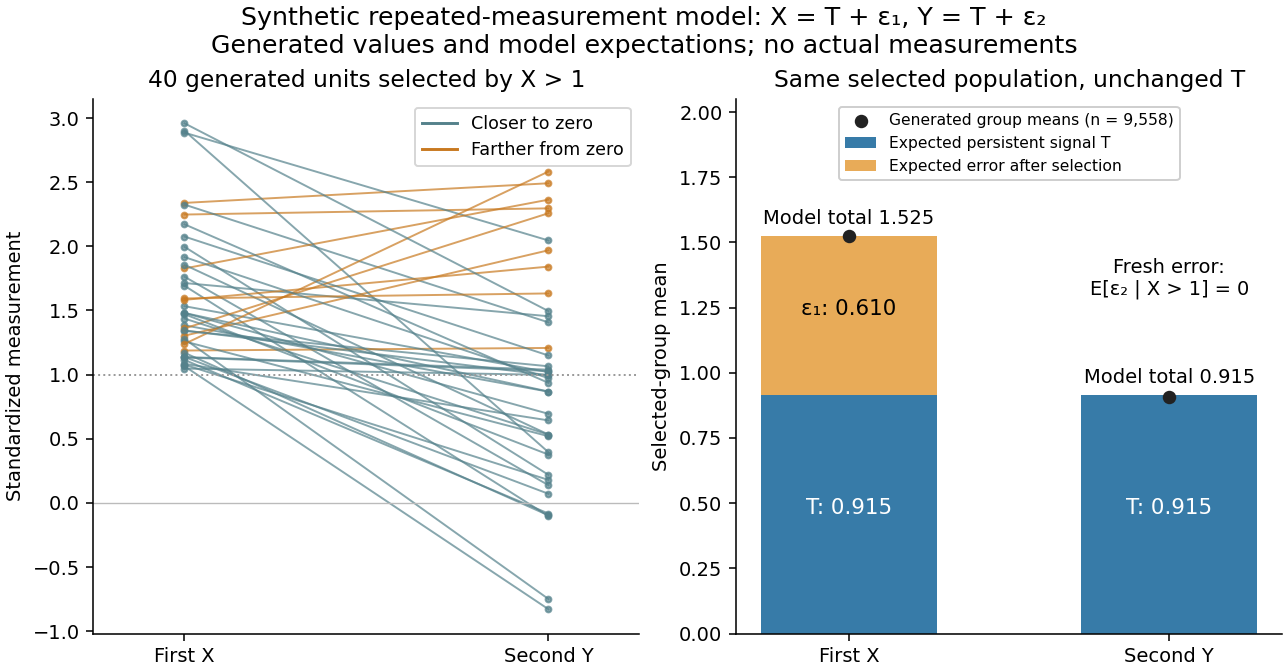
Select units with first reading , keep that membership fixed, and measure the same units again. The first reading now has a truncated normal distribution. For a general finite threshold , write for the standard normal density and for the standard normal distribution function. Since ,The tower property of conditional expectation lets us average the line over the selected group.[ref] At this givesThe average second reading is below the selection threshold even though every selected first reading exceeded it. This is a group expectation; any finite generated group's sample mean fluctuates around it. Selecting again on would define a different group and answer a different question.
The latent variable decomposition makes the apparent drop especially clear. Gaussian conditioning gives and . ThusThe first measurement error has zero unconditional mean, but positive selected mean. The second measurement error stays centered because it is independent of selection on . The persistent signal never changed.
For and a nonnegative integer , define the symmetric partial sum and its positive remainder bySuccessive omitted terms have ratio for . Bounding them by a geometric series givesConsequently the physical approximation to has error at most , while the dual approximation has error at most . The prefactor must be included when setting an absolute error tolerance.
For a truncation error below , at the physical side first passes this bound with : lattice points give , whereas gives . The dual side needs only . At the physical side needs only , whereas the dual side first passes the bound with : lattice points give . These counts measure symmetric lattice terms; using the even function symmetry reduces the distinct exponential function evaluations to . Truncation bounds do not include rounding error in a numerical implementation.
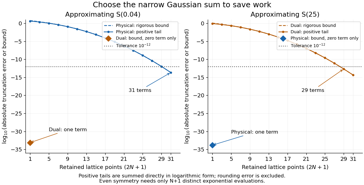
Positive Gaussian tails and rigorous bounds versus retained lattice points, showing the efficient side at reciprocal scales
. Details. In a Wheatstone bridge, the galvanometer connects the two comparison junctions. Its purpose is to locate a null measurement, rather than to measure the branch electric current through the unknown resistor. Using Wheatstone bridge detector loading and Thévenin's theorem, a settled moving-coil galvanometer with winding electrical resistance obeysHere is the bridge's open-circuit voltage and its Thévenin resistance. For a functioning passive detector with finite positive electrical resistances, exact implies , preserving Wheatstone bridge balance. Away from balance, the detector loads the junctions; its electrical resistance cannot be ignored.
For the illustrative , and a chosen , a bridge open-circuit voltage produces and . That lies inside the stipulated zero tolerance. The corresponding resolvable open-circuit voltage scale is about , not arbitrarily small. Actual limits also depend on the zero stability and calibration.
Use the detector checks in the slide-wire resistance bridge experiment: perturb the comparison to either side of the proposed balance and require opposite signs, while confirming the supply is on. A broken connection, a jammed pointer or an inactive supply can also give a zero reading. Conversely, a healthy bridge detector reads zero while the bridge arms still carry electric current. A zero deflection alone proves neither a broken conducting path nor infinite sensitivity.
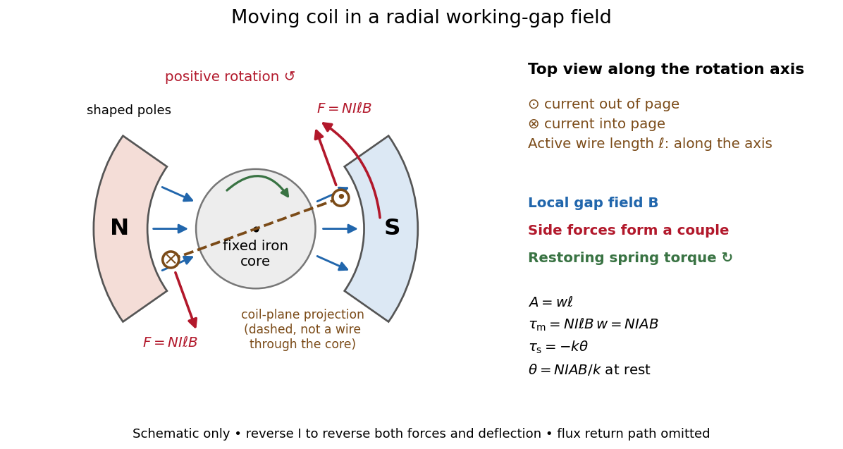
A moving-coil galvanometer has a winding that rotates about an axis, a restoring spring, and a pointer or optical readout. In the radial-field construction, a cylindrical iron core and shaped magnetic poles keep the magnetic field approximately in the coil's plane as it turns. The resulting moving-coil galvanometer torque is nearly independent of the deflection angle; the spring then converts electric current into a proportional settled deflection. [ref]
A moving-magnet galvanometer measures electric current through the torque it exerts on a movable magnetic dipole moment. A fixed coil carries the current and creates a magnetic field; a suspended magnet turns against a restoring torque supplied by its suspension or a reference field.
For sufficiently small deflections in a calibrated geometry, the coil field and resulting angular response are proportional to electric current. A pointer or reflected optical spot reads the angle. This differs from a moving-coil galvanometer, where the current-carrying coil itself moves. Mechanical damping determines whether the indication oscillates or settles smoothly after a current change.
Here Heun's method means the explicit endpoint-averaging Runge-Kutta method: take an Euler predictor , sample there, and average it with for the output. The second Runge-Kutta stage is evaluated at the predictor, not at the corrected endpoint. In particular it requires no implicit solve as the ODE trapezoidal rule does. Naming conventions vary between books; the formulas specify the method unambiguously.[ref]
Numerical solution of ordinary differential equations: One step methods by André Jürgen Massing. André Massing, Numerical solution of ordinary differential equations: One step methods, October 3, 2021, page 1, Example 1.1: Euler and Heun increment functions
For smooth , a Taylor expansion about gives , where is the state Jacobian matrix. Consequently the output is , matching the exact solution through degree two by the chain rule. This gives local truncation error and, with the usual bounded smoothness and Lipschitz continuity hypotheses on a fixed finite interval, global error . The Euler-Heun embedded pair compares this output with its Euler predictor.
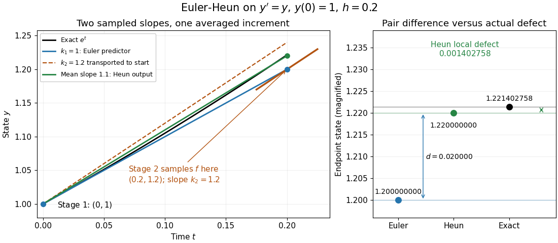
Euler-Heun stage geometry for y prime equals y: sample at the Euler predictor, then average slopes for the corrected endpoint
. Details. For , and , the sampled slopes are and . Transporting the second slope to the starting point would end at ; the average slope instead ends at . The exact exponential function reaches . The magnified endpoint comparison separates the pair difference from the actual Heun local defect .
Stipulate a model receiver held at with a reference at . Choose , so outward thermal conduction is . Ignore other heat transfer, take in both states, and stipulate perfect optical/electrical thermal equivalence. These values specify an original example; they are not measurements or claimed performance of a NIST instrument.
With the beam blocked, supply . With light admitted, the required heater power is . For stipulated radiometric absorptance at the chosen single wavelength,The illuminated receiver still gets of heating. The remaining of incident radiant flux escapes without heating it. Calling the measured heater reduction “incident power” would underestimate the stipulated incident radiant flux by .
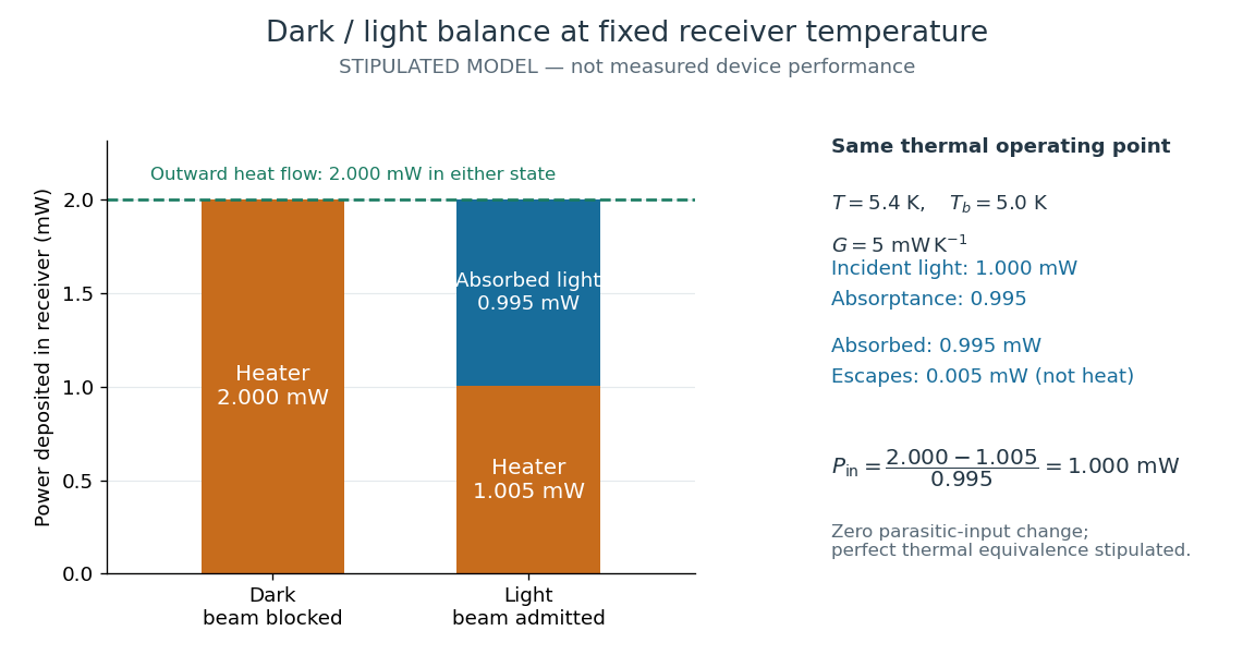
The same receiver temperature with different electrical and optical heating
. Original stipulated steady-state example, not experimental data. Both columns total of deposited heating and balance the same outward thermal conduction. Incident radiant flux is , of which is absorbed; the that escapes is outside the heating column. No response time or measured uncertainty is implied. Details.Two variations expose different pitfalls. First, if admitting the beam also adds of stray heating while the same is absorbed from the intended beam, the heater falls to . The apparent reduction is now ; subtracting recovers the beam's absorbed power. Second, keep the original heater readings but stipulate a light-state receiver offset at fixed reference temperature. The link carries an extra ; the inferred absorbed power becomes , and incident radiant flux becomes . This second variation deliberately violates exact fixed-temperature substitution.
The heater can supply only nonnegative power in this model. Consequently an absorbed beam above the available dark heater power cannot be compensated at the chosen setpoint merely by reducing the heater. The operating point, link, or admitted radiant flux must change; zero heater demand is a range boundary, not evidence of greater radiant flux sensitivity.
A radiometer thermal link is the intentional path for thermal conduction from receiver to reference block. Near a chosen operating point, write with local conductance in . A weaker link increases the steady temperature rise per added power, , but also increases the uncontrolled relaxation time when the link dominates other heat transfer. These are local linear approximations: actual thermal conductivity depends on temperature, and active feedback control introduces its own response. NIST explicitly describes the tradeoff between weaker links and smaller receiver heat capacity.[ref]
Pico-Watt ACR by National Institute of Standards and Technology. Key Design Features, final paragraph: response time proportional to receiver heat capacity and inverse thermal conductance
Pinned article: Introduction to the OurBigBook Project
Welcome to the OurBigBook Project! Our goal is to create the perfect publishing platform for STEM subjects, and get university-level students to write the best free STEM tutorials ever.
Everyone is welcome to create an account and play with the site: ourbigbook.com/go/register. We belive that students themselves can write amazing tutorials, but teachers are welcome too. You can write about anything you want, it doesn't have to be STEM or even educational. Silly test content is very welcome and you won't be penalized in any way. Just keep it legal!
Intro to OurBigBook
. Source. We have two killer features:
- topics: topics group articles by different users with the same title, e.g. here is the topic for the "Fundamental Theorem of Calculus" ourbigbook.com/go/topic/fundamental-theorem-of-calculusArticles of different users are sorted by upvote within each article page. This feature is a bit like:
- a Wikipedia where each user can have their own version of each article
- a Q&A website like Stack Overflow, where multiple people can give their views on a given topic, and the best ones are sorted by upvote. Except you don't need to wait for someone to ask first, and any topic goes, no matter how narrow or broad
This feature makes it possible for readers to find better explanations of any topic created by other writers. And it allows writers to create an explanation in a place that readers might actually find it.
Figure 1. Screenshot of the "Derivative" topic page. View it live at: ourbigbook.com/go/topic/derivativeVideo 2. OurBigBook Web topics demo. Source. - local editing: you can store all your personal knowledge base content locally in a plaintext markup format that can be edited locally and published either:This way you can be sure that even if OurBigBook.com were to go down one day (which we have no plans to do as it is quite cheap to host!), your content will still be perfectly readable as a static site.
- to OurBigBook.com to get awesome multi-user features like topics and likes
- as HTML files to a static website, which you can host yourself for free on many external providers like GitHub Pages, and remain in full control

Figure 2. You can publish local OurBigBook lightweight markup files to either OurBigBook.com or as a static website.
Figure 3. Visual Studio Code extension installation.
Figure 5. . You can also edit articles on the Web editor without installing anything locally. Video 3. Edit locally and publish demo. Source. This shows editing OurBigBook Markup and publishing it using the Visual Studio Code extension. 
- Infinitely deep tables of contents:




All our software is open source and hosted at: github.com/ourbigbook/ourbigbook
Further documentation can be found at: docs.ourbigbook.com
Feel free to reach our to us for any help or suggestions: docs.ourbigbook.com/#contact