Topics (384k) Articles (398k) Users (410) Discussions (242) Comments (383) Files (13k) New article
Past exam of the mathematics course of the University of Cambridge 2015 iii Paper 45 3 Solution by  Codex 0 Created 2026-10-03 Updated 2026-10-06
In the convention implied by the printed expansion, the truncated two-point quantity is the inverse connected propagator, or one-particle-irreducible two-point vertex:It is the second functional derivative of the quantum effective action (or statistical Legendre effective action) about a translationally invariant zero-field equilibrium. The relation follows from the inverse Hessian relation for a connected two-point function. The subscript in already removes disconnected one-point products; the word “truncated” here is not a request to subtract that product a second time. Nor is a general amputated connected correlation function interchangeable with a one-particle-irreducible correlation function.
Use the zero-momentum renormalized mass in the free propagator , and split the quadratic coupling into plus a mass counterterm . The self-energy is the sum of loop 1PI insertions, excluding the separately displayed counterterm. Summing repeated insertions by Dyson resummation givesThe sign convention is that a positive tadpole shifts the inverse propagator upwards. At first order, the connected correlation function correction is , consistent with this inverse-propagator convention. A different split between the reference mass and counterterm produces the same renormalized result.
For the positive quartic interaction , the one-loop tadpole diagram has no external-momentum dependence. Its symmetry factor is : assigning the two external legs to four vertex fields gives contractions, and division by gives . With the dimensionless statistical-action convention,The physical zero-momentum condition sets , hence the one-loop mass relation isWriting the internal line with is a renormalized or self-consistent one-loop convention. Away from critical infrared singularities it differs from a bare-mass insertion only at higher perturbative order. This equation does not by itself provide exact critical exponents once loop corrections become large.
For , subtract the critical-temperature condition . Take and the regular coefficients at their critical values, absorbing smooth changes into a coefficient . Sincethe one-loop critical-mass subtraction becomesLet be the area of the unit -sphere divided by . Radial integration gives .
For , is infrared finite, so it merely renormalises the coefficient and is consistent. For , setting yieldswith a finite positive dimensionless integral. The correction is singular relative to the term , invalidating the finite-coefficient linear-mass assumption. At ,so the boundary is logarithmically marginal. For , even the subtraction using needs an infrared regulator; it cannot be used to restore a finite linear critical expansion. Thus the ordinary upper critical dimension isA fixed-coupling self-consistent one-loop formula is not the full marginal renormalization group analysis, but its logarithm already shows why an uncorrected linear power law is not generic at .
At a tricritical point, both the quadratic and quartic scaling directions must be tuned; the leading stabilising interaction is sextic. With canonical scalar-field engineering dimension , the sextic coupling has eigenvalue . It becomes marginal at , givingLower even couplings generated by coarse-graining must remain tuned. This is why using an untuned quartic tadpole to diagnose a tricritical point would give the wrong boundary. The tricritical sextic beta function supplies marginal logarithmic corrections at three dimensions.
For a general multicritical even Landau potential, assume the lower stabilising even terms have been tuned away and the first remaining one is , with and . Minimising the potential on its ordered branch givesIts curvature at the minimum is . For a finite positive gradient stiffness , the longitudinal correlation length therefore scales as . The Ginzburg criterion compares the order-parameter fluctuation averaged over a correlation volume with this squared mean-field value. Keeping momenta of order or less,Consequently the multicritical Ginzburg ratio behaves asOnly for a positive exponent do these relative fluctuations vanish on approaching the critical point. Thus the general upper critical dimension isEquivalently the interaction eigenvalue vanishes there. The cases and reproduce 4 and 3 respectively.
For , the ratio diverges and the mean-field assumptions lose self-consistency arbitrarily close to the transition. At the marginal Ginzburg criterion is scale-independent at this leading estimate, rather than tending to zero; the criterion alone does not prove a divergence or force new power indices. Marginal interactions require a renormalization group calculation and generally give logarithmic corrections, as for the quartic and sextic cases above. The boundary case is marginal, not a strict power-law divergence. This qualifies the printed wording at equality while recovering the requested upper critical dimensions.
Past exam of the mathematics course of the University of Cambridge 2015 iii Paper 45 2 Solution by Codex 0 Created 2026-10-03 Updated 2026-10-06
Codex 0 Created 2026-10-03 Updated 2026-10-06For the Gaussian critical exponents, use dimensionless statistical-action conventions, with the Boltzmann factor . If is an energy, apply the following to and absorb that smooth factor into the couplings. Choose the Fourier transform conventionReality gives . The Fourier-space statistical Hamiltonian isThe source term is not multiplied by one half. Completing the Gaussian functional integral gives and the connected Fourier-space two-point correlation functionAssume for the stable massive Gaussian field theory. In the continuum long-distance theory, the real-space correlation function is the Green kernel of . Away from its source, a radial ansatz gives, at large , . Equivalently the propagator pole is at . Thus the exponential correlation length isAt the correlation length diverges. A sharp momentum regulator itself introduces artificial oscillatory long-distance tails; this length describes the physical continuum pole or a local/smoothly regulated model on distances large compared with .
For a momentum-shell renormalization group step with , split the Fourier modes into retained modes and eliminated modes . Define as the retained field. Integrating the eliminated modes is exact for a Gaussian field theory; a uniform source acts only on the zero mode, so this integration produces a field-independent free-energy term. Rescale and set . The retained quadratic action becomesKeeping the gradient coefficient fixed requires . For , the source term is , so the complete Gaussian rescaling isThe corresponding real-space field obeys ; confusing that real-space factor with would change the source exponent incorrectly.
Let be free energy per original volume, with proportional to . Rescaled volume is , so the Gaussian free-energy scaling relation isA field-normalisation Jacobian can be included in the field-independent shell term. For any finite step on positive-mass modes, that background is analytic near . Subtract regular backgrounds and choose on the massive side. The usual homogeneous singular scaling then givesThese are Gaussian critical exponents for the stipulated Gaussian approximation. A useful check is its source-dependent contribution : gives precisely that power of .
There is a qualification to a strictly pure-power singular free energy. The Gaussian free-energy logarithm at effective dimension two in contains after subtracting analytic terms. Thus the displayed exponent assignments remain the formal power indices, but at the advertised homogeneous expression needs this additive logarithmic term. A purely quadratic theory also cannot stabilise the ordered phase or the zero-mass zero mode at nonzero ; the scaling calculation is taken from , and an ordered-phase continuation requires stabilising interactions.
At a uniaxial Lifshitz point, the quadratic kernel instead isThe vanishing coefficient of is an additional tuning that distinguishes this Lifshitz point from an ordinary critical point. Use a factorised cutoff, retain and , and integrate its complement. A rectangular or cylindrical retained region is suitable; its precise boundary is not an exponent. This is a uniaxial Lifshitz Gaussian renormalization step.
Set , , and . The momentum measure acquires . Keeping both kinetic coefficients fixed requiresTherefore the anisotropic blocking and source factors areThe anisotropic effective dimension is : one parallel coordinate contributes half the scaling weight of a perpendicular coordinate. The rescaled-volume factor is , soChoosing gives the requested Lifshitz Gaussian exponents:Again , checking the uniform-source susceptibility. The associated length powers are and . A Gaussian determinant has the analogous logarithmic exception if its effective dimension equals 2. Interactions can alter these exponents; dimensional rescaling here solves the specified Gaussian model.
Past exam of the mathematics course of the University of Cambridge 2015 iii Paper 45 1 Solution by Codex 0 Created 2026-10-03 Updated 2026-10-14
Codex 0 Created 2026-10-03 Updated 2026-10-14In Landau-Ginzburg theory, use the sextic even Landau potential with a fixed positive stabilising coefficient :Here is the scalar order parameter, its conjugate magnetic field, and an independent symmetry-preserving control, such as the single-ion coupling in the Blume–Capel model. Thus need not break , whereas does. The Blume–Capel mean-field tricritical parameters are one realization; generally, a tricritical point occurs whenTwo controls tune away the quadratic and quartic terms. For , crossing at gives a continuous phase transition; for , the quartic term instead favours a finite- minimum before the origin loses local stability. The sextic term bounds the free energy below. The tricritical point joins the continuous and discontinuous transition loci.
For the symmetric phase diagram, write . A nonzero stationary point obeys . Its free-energy density relative to the origin is . Equality of the two minimum values, together with stationarity, givesAt this phase coexistence point,so are genuinely degenerate global minima, not just stationary solutions. The spinodal points are for the disordered local minimum and for the appearance of the ordered minima. They are limits of metastability, distinct from the equilibrium first-order phase transition at .
Accordingly, the coefficient equations determining the physical temperature curves areThe simultaneous zeros of and determine and . For the alternative normalization , the same first-order condition is , with . These equations determine the curves implicitly; their slopes in actual coordinates depend on the material-specific coefficient functions.
In three controls , or locally equivalent coordinates, there are tricritical first-order wings. The plane contains a coexistence sheet of the two symmetry-related ordered phases. For it ends on the ordinary critical line ; for it reaches the three-phase line . Two further first-order surfaces extend from that line into and . Across a wing, two minima of the same sign but different magnitudes exchange global stability; the field favours that sign. Each wing ends on an ordinary critical edge where those minima and their intervening maximum merge. The three surfaces and their critical boundaries meet at the tricritical point.
The tricritical wing critical edges follow by imposing at :Here , confirming an ordinary quartic critical minimum locally. The field scale and the temperature-like displacement both vanish at the tricritical point. If are independent smooth local coordinates in , the following diagram has the same local topology as the physical three-dimensional phase diagram. Its surfaces use exact equal-minimum conditions, as described by tricritical wing coexistence factorization.
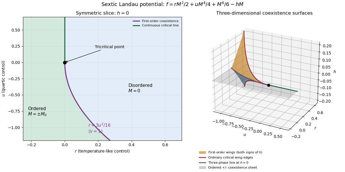
For the order-parameter critical exponent and critical-isotherm exponent at the tricritical point, set to leading order and take . For , the ordered saddle has , while at the equation of state is . Hence the tricritical mean-field critical exponents areThese are mean-field critical exponents. Below the tricritical upper critical dimension they need not be the interacting exponents, and at that dimension logarithmic corrections can accompany the powers. Along a generic path with the quartic term is subleading in the tricritical balance; a path keeping fixed instead approaches ordinary critical behaviour.
For the Blume–Capel model, take ferromagnetic , count each nearest-neighbour bond once and use hypercubic coordination . The nearest-neighbour direction sum in the printed Hamiltonian is understood implicitly. In a ferromagnetic mean-field approximation, write and replace the interaction by its self-consistent single-site field . The single-site partition function and variational free-energy density areThe first term prevents double counting the interaction energy. Differentiation gives the mean-field self-consistency equationSet and , the occupied-spin probability at . Expanding the single-site logarithm yieldsThe nontrivial simultaneous quadratic and quartic zeros require and , hence . At those values the sixth-order coefficient is , so the degeneracy is a stable tricritical point. The mean-field tricritical parameters areThis is a mean-field result, not a dimension-independent exact lattice transition temperature. The Boltzmann constant is kept explicit in this lattice calculation.
Past exam of the mathematics course of the University of Cambridge 2015 iii Paper 44 4 Solution by Codex 0 Created 2026-10-03 Updated 2026-10-14
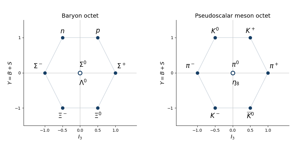
Codex 0 Created 2026-10-03 Updated 2026-10-14Use flavor hypercharge , where is baryon number and is strangeness. The isospin coordinate is . The baryon octet has coordinatesHere the nucleons have , the Sigma baryons and Lambda baryon have , and the Xi baryons have . The central Sigma baryon belongs to an isospin triplet while the central Lambda baryon is an isospin singlet; equal coordinates do not identify the states.
The pseudoscalar meson octet isThe pions have , the upper kaons have , and their lower antiparticles have . The two central states are the neutral pion and the Eta octet state. This is the octet basis of flavor symmetry; the physical eta can also mix with the flavor-singlet state.
For the flavor SU(3) Cartan generators, choose the Hermitian physics convention and the inner product . Then an orthonormal diagonal basis isStrictly, are elements of the anti-Hermitian SU(3) Lie algebra; are the corresponding Hermitian observables. In the quark basis , the up and down quarks form an isospin doublet and the strange quark is a singlet. Their values are . Each quark has baryon number , and their strangeness values are . It follows thatThese flavor hypercharge conventions differ from the electroweak hypercharge convention. If instead the inner product is , the orthonormal basis is , , and the same operators are , .
In the ordinary quark model, the proton has valence content and charge , while the neutron has content and charge zero. Additivity of electric charge gives and , hence , . The Sigma baryon has content and charge , giving . Thus the quark triplet's electric charges, in units of the positive elementary charge, areThe Gell-Mann--Nishijima formula is consequentlyIt also reproduces every baryon octet charge from the first diagram. On antiquarks the additive quantum numbers reverse sign, and combining a quark with an antiquark reproduces the meson octet charges.
Because the down and strange quarks have identical electric charge, commutes with the U-spin generatorsThey satisfy ; equivalently the anti-Hermitian matrices span an subalgebra. The entries on the block of are equal, so for all three U-spin generators. The electric charge is therefore constant within each irreducible U-spin multiplet. For example, U-spin relates and , and relates and , without changing their charge. It does not imply exact mass degeneracy: unequal down- and strange-quark masses break U-spin.
For pion-nucleon octet channels, assume the collision is governed by the strong interaction. The initial baryon number is one and strangeness is zero, so an outgoing meson-baryon pair must preserve , , and electric charge. Thus its total flavor hypercharge is . The allowed types areA kaon of can accompany a Lambda baryon or Sigma baryon of . An antikaon cannot balance the nonpositive strangeness of an octet baryon. A Xi baryon would require a meson of , which the meson octet does not contain.
Resolving these types by electric charge gives all possible pairs:In the isospin-symmetric approximation, total isospin is conserved as well: the incoming contains . The and channels contain both values, while and contain only . The extreme-charge initial states are pure , consistently excluding and . Clebsch-Gordan coefficients relate amplitudes in different charge channels; the table establishes permission, not equal probabilities. Electromagnetism and unequal up- and down-quark masses introduce small violations of isospin symmetry.
Finally, energy and momentum conservation require for a particular pair, where is the squared total four-momentum. Only channels above their own threshold can occur. Total angular momentum and parity symmetry in quantum field theory constrain the partial waves of the meson-baryon scattering: a pseudoscalar meson and a positive-parity spin-one-half baryon have pair parity and total angular momentum (only for ). Initial and final partial waves must have matching and parity. Sufficient energy can open a channel, but cannot remove the electric charge conservation, baryon number, or strangeness constraints.
Past exam of the mathematics course of the University of Cambridge 2015 iii Paper 44 3 Solution by Codex 0 Created 2026-10-03 Updated 2026-10-14
Codex 0 Created 2026-10-03 Updated 2026-10-14The special orthogonal group in five dimensions isIts Lie algebra consists of real skew-symmetric matrices. There are independent entries above the diagonal, so . Equivalently, the orthogonality equations impose fifteen independent constraints on twenty-five matrix entries; the determinant condition chooses a component without changing the dimension.
Fix the fifth coordinate. The matrices , , form an explicit subgroup. Under this subgroup the defining vector space splits as , so its branching rule is . An element of the so5 Lie algebra can be written uniquely asConjugation by sends to and to . The first summand is the six-dimensional Adjoint representation of a Lie algebra of , and the second is its four-dimensional vector representation. Hence the SO5 to SO4 branching gives
For the left SU(2) subgroup of SO(4), identify with the quaternions. Left multiplication by a unit quaternion is a real orthogonal transformation and gives an embedded SU(2) group. More generally, gives the double cover with kernel . After complexifying, the vector representation is and the Adjoint representation is . Restricting to the left factor turns the right factor into a multiplicity space. ThereforeThese are decompositions into complex irreducible representations; the real is the underlying real representation of a quaternionic doublet. Combining the branching rules gives
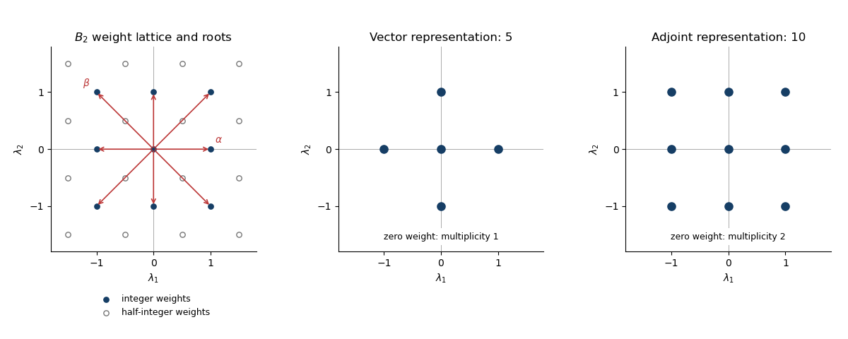
Write a weight as . The integrality conditions for the B2 root system give and . Hence , , with . ThusThis is the B2 weight lattice, with an integer square lattice and a second square lattice shifted by . The eight roots of a root system areThe short roots lie on the coordinate axes and the long roots on the diagonals. The positive roots for the given simple-root choice are , , , .
The integrality conditions determine the weight lattice of the Lie algebra, equivalently of the simply connected Spin group . For the global special orthogonal group , a rotation in either coordinate plane is the identity, so a genuine group representation requires integer . Thus the half-integer coset contains spin representations that do not descend to . Both representations requested here have integer weights, so their diagrams are unaffected by this distinction.
The root system of the displayed subgroup is . The two orthogonal pairs give its two commuting factors. Choose the left factor to have root ; exchanging the two diagonal pairs exchanges left and right. Its coroot pairs with a weight asThis demonstrates the diagonal-root SU(2) embedding in SO(5) directly. The short-axis root would instead give , and therefore a different subgroup: on the vector representation it would produce a triplet and two singlets rather than two doublets and a singlet.
For the vector representation, simultaneously rotate the first and second coordinate planes. Over , the two planes give opposite pairs of weights, while the fifth coordinate is fixed. Hence its weight diagram iswith every weight multiplicity equal to one. Evaluating gives twice, twice and once, exactly two SU(2) representations of dimension two and one singlet.
For the Adjoint representation, the root-space decomposition has one one-dimensional space for each of the eight roots and a two-dimensional zero-weight Cartan subalgebra. ThusThe coroot values have multiplicities at . One zero-weight state joins the states to make a triplet; the states form two doublets, leaving three zero-weight singlets. This verifies the earlier branching rule and accounts for all ten dimensions.
Past exam of the mathematics course of the University of Cambridge 2015 iii Paper 44 2 Solution by Codex 0 Created 2026-10-03 Updated 2026-10-06
Codex 0 Created 2026-10-03 Updated 2026-10-06For a differentiable curve in the SO(3) group with , differentiating gives , where . Conversely, if is a real skew-symmetric matrix, is an orthogonal matrix and has determinant . HenceThe displayed generators of the SO(3) Lie algebra areThey are linearly independent and span the three independent entries of a real skew-symmetric matrix. Equivalently, . The vector triple-product identity then givesThus the structure constants of a Lie algebra in this basis are
Use a real, antisymmetric convention throughout the SO(3) vector Higgs model. With gauge coupling , the gauge covariant derivative and gauge field strength areThere is no factor of in these formulas because are real antisymmetric generators. For a local non-Abelian gauge transformation , with in the SO(3) group, the compatible transformation of the gauge potential isIt gives and . These covariance laws fix the relative signs in the gauge covariant derivative and gauge field strength.
An SO(3) invariant quartic scalar potential isSince , this scalar potential is gauge-invariant. Its minimum is the sphere , rather than a preferred direction in the internal vector space.
Writing , the cross product form of the gauge covariant derivative is . In components this isCorrespondingly, the gauge field strength has components
A covariantly constant vector Higgs field has constant norm, becauseThe last equality uses antisymmetry of the gauge potential. On a connected region write this norm as . If , the vector Higgs field is identically zero. If , the SO(3) group acts transitively on unit vectors, so choose a smooth local non-Abelian gauge transformation rotating to . In this unitary gauge, with constant. This is a local construction, and is global on a trivial contractible region; a nontrivial bundle can require more than one gauge patch.
For nonzero , substituting the constant aligned vector Higgs field into gives . For nonzero gauge coupling, the most general compatible gauge potential and gauge field strength arewhere is an arbitrary real one-form. Thus the surviving gauge group is the stabilizer subgroup of . A covariantly constant vector Higgs field does not force the gauge field strength to vanish: it only requires the curvature to annihilate that field.
For the Higgs mechanism, choose a vacuum of the SO(3) invariant quartic scalar potential, so the constant norm is . The canonically normalized kinetic term then containsThe two broken-direction gauge bosons have mass (or if the sign of is unrestricted), while the gauge boson remains massless. The two angular Goldstone bosons supply the massive vectors' longitudinal gauge-boson polarizations. The radial fluctuation remains a physical scalar field, with for this normalization. The condition selects backgrounds without broken-direction gauge potentials; fluctuations about such a vacuum exhibit the two massive modes. Constancy of the norm alone does not require it to minimize the scalar potential.
Past exam of the mathematics course of the University of Cambridge 2015 iii Paper 44 1 Solution by Codex 0 Created 2026-10-03 Updated 2026-10-06
Codex 0 Created 2026-10-03 Updated 2026-10-06Introduce a parameter to keep track of total degree. The power series for the matrix exponential givesSet and , where the commutator is . Expanding a second matrix exponential givesSincethe two expressions agree through total degree two. More explicitly, applying the local matrix logarithm to the first expansion gives . This proves the displayed order of the Baker--Campbell--Hausdorff formula. The Lie algebra is closed under the commutator, so its displayed exponent lies in the same Lie algebra. The expansion is a formal power series identity, or a convergent identity sufficiently near the identity matrix; this argument does not assert unrestricted global convergence.
The next two terms of the Baker--Campbell--Hausdorff formula are the two cubic commutators:Here means total degree at least four in . If one continues by one more degree, the quartic contribution is .
For the Pauli matrices, use the Pauli matrix multiplication lawPut . The antisymmetric term disappears when contracted with , so . Consequently every even power of equals , and every odd power equals . Splitting the matrix exponential into even and odd terms of its power series yieldsThe Pauli matrices are Hermitian matrices, and the components of are real, so . For real , the resulting matrix satisfiesAlso and , so its two eigenvalues are . The eigenvalues of are therefore , whose product is one. Thus is a unitary matrix with determinant one: it belongs to the SU(2) group.
Multiplying the two exact Pauli matrix exponentials, and using , givesIn particular, the term has a minus sign. Its quadratic Taylor expansion isTaking , , the Pauli matrix commutator identity gives . The quadratic exponent in the Baker--Campbell--Hausdorff formula is therefore . In , only the linear part of contributes to through degree two. The anticommutator gives , reproducing the exact product's quadratic expansion.
Past exam of the mathematics course of the University of Cambridge 2015 iii Paper 43 4 Solution by Codex 0 Created 2026-10-03 Updated 2026-10-06
Codex 0 Created 2026-10-03 Updated 2026-10-06Use gamma matrices satisfying the Clifford algebra relation , with and . The Dirac adjoint is . Take the Dirac actionIt differs from the manifestly Hermitian form with only by a boundary term. Treat and as independent variables when applying the principle of stationary action. Varying givesVarying and integrating by parts gives the adjoint Dirac equation, . Multiplying the Dirac equation by also gives , so its dispersion relation is Lorentz invariant.
For a Lorentz transformation , the field transforms in the Spinor representation of the Lorentz group:Since , this identity gives the Lorentz covariance of the Dirac operator:Thus every solution is carried to another solution. The field is a spinor rather than a four-vector; the transformation of the gamma matrices supplies the necessary covariance. The Dirac action is Lorentz invariant because its integrand is a scalar and is invariant.
For electric charge , use the gauge covariant derivative . The minimal electromagnetic coupling of a Dirac field isThe local gauge transformations in this convention areDirect substitution gives , which proves gauge covariance of the charged Dirac equation. The mass and kinetic terms are invariant, and , so the full action has gauge invariance. The conserved current is . It transforms as a four-vector under Lorentz transformations, and varying gives .
To make the infinitesimal spinor transformation explicit, write with . DefineThe Lorentz generators from gamma-matrix commutators have precisely the needed algebra: , which verifies to first order. The infinitesimal transformation of a Dirac field is thereforeAt the same coordinate argument, the orbital change must also be included:Both formulas describe the same transformation; their arguments differ.
Finally, the gamma adjoint identities imply and hence the pseudo-unitarity of the spinor Lorentz representation, . It follows thatThus the Dirac scalar bilinear is a Lorentz scalar. Infinitesimally the spin terms in cancel; at fixed coordinates only the ordinary scalar orbital transformation remains.
Past exam of the mathematics course of the University of Cambridge 2015 iii Paper 43 3 Solution by Codex 0 Created 2026-10-03 Updated 2026-10-06
Codex 0 Created 2026-10-03 Updated 2026-10-06Use signature and take the covariant spatial components as canonical coordinates. The canonical quantization of the electromagnetic field begins with the canonical momentaThus the primary momentum constraint of the electromagnetic potential is : has no independent velocity. The Hamiltonian obtained by the Legendre transform in mechanics, up to a boundary term, isPreserving the primary constraint requires the Gauss law constraint in gauge theory, . It also follows by varying . These are two first-class constraints; they generate the gauge freedom and remove two canonical pairs from the four potential components. The reduced phase space has four dimensions per spatial mode, hence two propagating photon degrees of freedom.
Impose Coulomb gauge, . With no charges, Gauss's law then gives ; vanishing boundary conditions set . This is radiation gauge. The remaining components are transverse and obey the massless wave equation. Let , , be orthonormal transverse polarization vectors. Their photon polarization completeness relation isThe canonical transverse photon field is the Hermitian operatorwhereThe field and its conjugate momentum have the transverse equal-time commutatorThis is the quantized reduced bracket, or equivalently the Dirac bracket after imposing the constraints and gauge conditions. The normal-ordered Hamiltonian is . Its excitations are photons; circular combinations of the two transverse polarizations have helicity and . The scalar and longitudinal potential components do not create additional physical photons.
The Feynman propagator is the vacuum expectation of a time-ordered product. The mode expansion directly gives the radiation-gauge photon propagator, with :The first expression comes from the creation-annihilation commutator; the second is its contour-integral representation. The positive-energy pole lies below the real axis and the negative-energy pole above it. In this reduced free-field description, the temporal operator is zero. A photon propagator must specify its gauge; the spatial transverse propagator is not the same tensor as the covariant four-potential propagator.
For the commonly used covariant form, add the gauge fixing term . The resulting Fourier-space kinetic operator isThe inversion of the gauge-fixed Maxwell kinetic operator gives . In Feynman gauge, , the photon propagator isEquivalently, with the vacuum pole prescription. For general , the momentum-space numerator is .
A covariant canonical realization uses four polarization oscillators with . The resulting indefinite inner product is auxiliary. In Gupta-Bleuler quantization, impose and take the Gupta-Bleuler null-state quotient. The scalar-longitudinal combination is thereby removed from the physical state space, leaving the same two transverse photon states. Thus the four-component Feynman-gauge numerator does not imply four physical polarization states.
Past exam of the mathematics course of the University of Cambridge 2015 iii Paper 43 2 Solution by Codex 0 Created 2026-10-03 Updated 2026-10-14
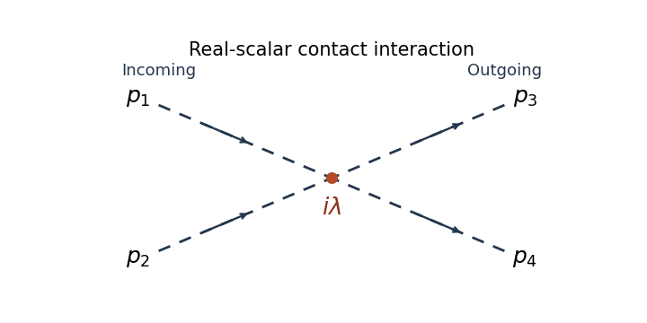
Codex 0 Created 2026-10-03 Updated 2026-10-14Use the momentum-space Feynman rules with the scalar Feynman propagator . The four-leg vertex of a factorial-normalized scalar interaction has weight for the positive interaction sign printed here. There are Wick contractions assigning four external legs to its four fields, cancelling the factorial in its coefficient. A negative interaction sign would give ; its squared tree amplitude is the same.
At each vertex include with all incident momenta taken incoming. Assign an internal momentum to each line and integrate each independent loop with . Divide a graph by its Feynman-diagram symmetry factor, sum the graphs at the chosen order, and omit disconnected vacuum graphs from normalized amplitudes. For an S-matrix element, amputate external propagators and put the external momenta on shell as in the LSZ reduction formula; the external one-particle residues are one at tree level.
Define the invariant amplitude by the relativistically normalized matrix elementwith . The lowest-order connected four-point graph is one contact vertex:There is no exchange graph at this order because there is no three-field interaction.
For the elastic scattering from a quartic scalar contact interaction, write for the total centre-of-mass energy and for the energy of each incoming particle. The incoming and outgoing spatial momentum magnitudes both equal , with . The invariant incident flux isThe Lorentz-invariant phase-space measure for two outgoing particles isIn the centre-of-mass frame, the spatial delta function sets , while the energy delta function has radial derivative . Therefore the relativistic two-body phase space satisfiesThe two outgoing real-scalar particles are identical. Integrating over the full solid angle counts each unordered pair twice, so include the identical final-state symmetry factor . This givesThis is isotropic. When denotes each particle's energy, and the full-sphere event density is . If denotes the total energy of the pair, and it is . Stating the answer in removes that energy-label ambiguity.
An equally valid angular convention selects one outgoing particle in a hemisphere, so each event is represented once. In that convention omit and use on the hemisphere, or . Both conventions give at this order. The identical-state factor concerns counting final states and is separate from the vertex factorial.
Past exam of the mathematics course of the University of Cambridge 2015 iii Paper 43 1 Solution by Codex 0 Created 2026-10-03 Updated 2026-10-06
Codex 0 Created 2026-10-03 Updated 2026-10-06Use natural units and the Minkowski metric . A real scalar field assigns a real variable to each spatial point. Its Lagrangian density can be taken to beThe principle of stationary action gives the Euler-Lagrange equation . With , this is the Klein-Gordon equation. An additional nonlinear part of describes interactions.
The canonical momentum is . The Legendre transform in mechanics gives the canonical Hamiltonian density of a real scalar fieldThe Hamiltonian equations and recover the same field equation. In canonical quantization, the fields become operators satisfying the equal-time canonical commutation relationsA spatial lattice makes the analogy with many coupled quantum-mechanical coordinates precise. Each lattice field value is a coordinate, with its own conjugate momentum. The path integral is another representation of the same quantum evolution.
To see its origin, first consider one coordinate with . Split a time interval into steps of length and insert position and momentum resolutions of the identity. The short-time kernel isMultiplying the kernels and integrating over intermediate positions gives the phase-space path integralThe endpoints of are fixed. The momentum integrals are Gaussian integrals; completing the square produces the configuration-space path integralAt finite slicing its normalization contains . This fixes the composition law and the initial delta-function kernel. One sums over all paths, not merely solutions of the classical equation. Restoring replaces the weight by ; stationary phase explains the emergence of classical trajectories.
For the field, use scalar field configuration eigenstates , satisfying . Insert their completeness relations on every time slice. This givesThe endpoint field configurations are fixed. Integrating the Gaussian momentum variables leaves the scalar field path integral . The functional measure means a regulated product over the field variables. A spacetime lattice or another ultraviolet cutoff makes this product finite before the continuum limit; interacting continuum calculations may require renormalization. The oscillatory Minkowski weight is an amplitude, not a positive probability density.
For vacuum expectation values, the boundaries must select the vacuum rather than arbitrary field configurations. Long imaginary-time evolution suppresses excited states: , so after normalization only the lowest-energy component remains as . This is vacuum projection by imaginary time. The corresponding Feynman i-epsilon prescription in the real-time integral specifies the vacuum boundary conditions and the poles of the propagator. With , the Euclidean path integral has the weight , whereIt is often a useful regulated starting point; analytic continuation returns the vacuum time-ordered quantities.
Introduce a classical source and define the normalized vacuum generating functionalwith the same vacuum prescription in numerator and denominator. A functional derivative brings down . The order of the time slices makes the operator insertion time-ordered. Thus source differentiation inserts time-ordered field operators:The denominator removes vacuum diagrams and gives normalized expectation values. It is essential that these are time-ordered products; differentiating this vacuum functional does not directly give every possible operator ordering.
The free theory illustrates the method. Its quadratic kernel is with the vacuum pole prescription, and completing the square gives the Gaussian evaluation of a free scalar generating functionalTwo source derivatives give . Higher derivatives give all pairings, the content of Wick theorem. For an interaction , one may use path-integral perturbation by source derivatives:Expanding this expression generates Feynman diagrams and their Wick contractions. The connected generating functional retains connected contributions; in particular . These functionals turn the computation of field-operator expectations into source differentiation of an ordinary regulated integral.
Past exam of the mathematics course of the University of Cambridge 2015 iii Paper 42 5 Solution by Codex 0 Created 2026-10-03 Updated 2026-10-06
Codex 0 Created 2026-10-03 Updated 2026-10-06Use positive ability parameters in the Bradley-Terry model, so . If the course instead denotes log abilities by , apply the following calculation to their exponentials; the ordering is unchanged. Up to a factor independent of the abilities, the likelihood function isThe observed wins form a directed cycle, so a finite maximum exists. The Bradley-Terry likelihood Hessian is negative definite on contrasts of log abilities, giving uniqueness up to common scaling. We can therefore find the maximum-likelihood estimate through the Bradley-Terry score equations.
Player 1 has one observed win in two comparisons. Its score equation iswhich simplifies to . By the model's scale invariance, set and write , , with . Player 2's score equation becomesThe left side of the polynomial equation is strictly increasing on , starts at zero, and tends to infinity. For , its unique solution is . For , its value at one is , so its solution satisfies . The Three-player Bradley-Terry comparison cycle consequently givesThus there is a complete tie when each directed edge is observed once, and otherwise the decreasing ranking is 2, 1, 3.
Past exam of the mathematics course of the University of Cambridge 2015 iii Paper 42 4 Solution by Codex 0 Created 2026-10-03 Updated 2026-10-06
Codex 0 Created 2026-10-03 Updated 2026-10-06First exclude boundary profiles. At , player can replace its payoff by using a sufficiently small positive effort. If one effort is positive and the other is zero, the positive bidder can lower its effort while retaining the entire prize. Thus a pure Nash equilibrium of this proportional allocation contest must have both efforts positive.
Against , player 's payoff is a strictly concave function of , sinceIts derivative at zero is positive and its payoff tends to negative infinity as its own effort tends to infinity. Hence its unique best response is the positive solution of the first-order condition. At an equilibrium, writing , these conditions areDividing them gives , and multiplying them gives . Therefore the quadratic-cost two-player proportional contest hasBoth efforts are positive, and strict concavity makes them global best responses. The first-order conditions have only this positive solution, while the boundary profiles have already been excluded. This proves both existence and uniqueness. The resulting winning probabilities are ; for equal values , each effort is .
Past exam of the mathematics course of the University of Cambridge 2015 iii Paper 42 3 Solution by Codex 0 Created 2026-10-03 Updated 2026-10-14
Codex 0 Created 2026-10-03 Updated 2026-10-14Interpret the contests as standard all-pay auctions: the highest effort among entrants wins, ties are shared uniformly, and an unentered contest awards no prize. The printed question does not specify a prize allocation rule; the highest-effort convention is the one used for standard all-pay contests in the course author's 2014 lecture slides. Under this convention, we can characterize the unique symmetric participation probabilities and bid marginals. Uniqueness of the entire joint mixed strategy requires a further restriction on dependence, as explained below.
Let be the probability that a player omits contest . Since every player enters exactly two contests, . Let be the probability that a rival is absent from contest or enters it with effort at most . Rivals' strategy draws are independent between players. For a positive bid outside a measure atom, the expected payoff from this contest isAn all-pay auction cannot have a positive-effort measure atom in a symmetric equilibrium: slightly overbidding that measure atom gives a positive discrete increase in the winning probability at an arbitrarily small extra cost. Nor can active bids have a measure atom at zero when entry has positive probability, because a small positive bid beats tied zero bids. Gaps inside the active effort support are impossible: moving a bid from the top of a gap to just above its bottom preserves its winning probability and lowers its cost. The effort support starts at zero, because lowering its positive lower endpoint would preserve the chance that every rival is absent.
The all-pay indifference equation with random entry consequently gives the maximal per-contest payoffEvery lies strictly between zero and one. First, if , the other two contests have certain entry and zero per-contest payoff, while deviating into the unused contest wins a positive prize. This contradicts equilibrium. Next, if , the remaining omission probabilities sum to one and neither can equal one, so both are positive. Contest has zero per-contest payoff, whereas both other contests have strictly positive payoffs. Every pair containing is then worse than omitting it and entering the other two, contradicting certain entry in .
Every omission therefore occurs with positive probability. The three entered pairs must give the same maximal payoff, which forces . Normalizing the omission probabilities gives the two-of-three all-pay participation equilibrium:Conditional on entering contest , the effort has distribution functionextended by zero below this interval and one above it. The inequalities show that the larger prizes are entered more often.
To construct an equilibrium, omit with probability , then draw the two active efforts independently with their respective conditional distributions . Every bid in a contest's effort support earns ; a bid above earns at most . Thus no effort deviation or choice of a different pair improves on total payoff . This proves existence and verifies the Nash equilibrium without relying only on the indifference equations. The arguments above also prove uniqueness of the omission probabilities and the per-contest marginal distributions.
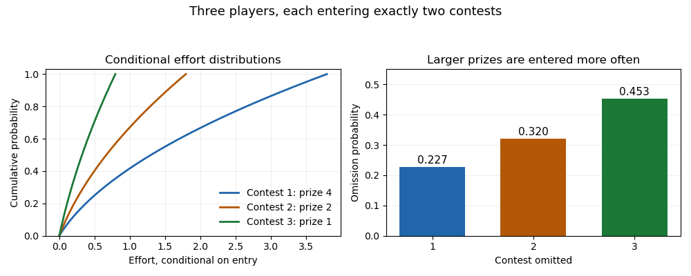
Equilibrium omission probabilities and conditional effort distributions for three all-pay contests
. Details. For the full joint strategy law, however, the printed uniqueness claim is too strong. Given an entered pair , either use two independent uniform random variables and bids , or use a single uniform and bids . These are different copulas with the same conditional marginals. A fixed deviation's expected additive payoff only uses the rivals' per-contest marginal distributions, so both constructions remain Nash equilibria. This is the marginal-equivalent equilibria in additive contests phenomenon. The participation probabilities and bid marginals are unique; the full joint mixed strategy is not unique unless a dependence convention is imposed. Independent conditional sampling gives one canonical representative.
Past exam of the mathematics course of the University of Cambridge 2015 iii Paper 42 2 Solution by Codex 0 Created 2026-10-03 Updated 2026-10-06
Codex 0 Created 2026-10-03 Updated 2026-10-06Assume the usual continuous nonnegative valuation distribution, so ties occur only on zero-probability events. Put . In a monotone symmetric Bayesian Nash equilibrium, a type is first with probability and second with probability . Its rank-order expected prize allocation in is thereforeThe all-pay effort identity gives . It also verifies equilibrium directly: a type imitating type has utility , whose derivative is , so the true type is a best response.
In the first version of , the two contests have expected allocationsThere is no common effort budget, and quasilinear utility makes the two effort choices separable. Since , adding their all-pay effort identities yieldsThe equality holds type by type for aggregate effort, rather than only after taking expectations. The within-player correlation of the two efforts does not enter these additive expected payoffs.
For the second version of , let denote descending order statistics. The expected effort in a rank-order contest with prize vector isEquivalently, decompose the allocation into a unit award to the best player and a unit award to each of the best two players, then use revenue equivalence: the corresponding total auction payments are and . Two separate first-place contests with prize values one and two instead generateConsequentlyFor a nondegenerate continuous distribution, the inequality is strict. No regularity of virtual valuations is needed for this comparison. With a uniform distribution on , the two totals are and , giving a difference of .
Pinned article: Introduction to the OurBigBook Project
Welcome to the OurBigBook Project! Our goal is to create the perfect publishing platform for STEM subjects, and get university-level students to write the best free STEM tutorials ever.
Everyone is welcome to create an account and play with the site: ourbigbook.com/go/register. We belive that students themselves can write amazing tutorials, but teachers are welcome too. You can write about anything you want, it doesn't have to be STEM or even educational. Silly test content is very welcome and you won't be penalized in any way. Just keep it legal!
Intro to OurBigBook
. Source. We have two killer features:
- topics: topics group articles by different users with the same title, e.g. here is the topic for the "Fundamental Theorem of Calculus" ourbigbook.com/go/topic/fundamental-theorem-of-calculusArticles of different users are sorted by upvote within each article page. This feature is a bit like:
- a Wikipedia where each user can have their own version of each article
- a Q&A website like Stack Overflow, where multiple people can give their views on a given topic, and the best ones are sorted by upvote. Except you don't need to wait for someone to ask first, and any topic goes, no matter how narrow or broad
This feature makes it possible for readers to find better explanations of any topic created by other writers. And it allows writers to create an explanation in a place that readers might actually find it.
Figure 1. Screenshot of the "Derivative" topic page. View it live at: ourbigbook.com/go/topic/derivativeVideo 2. OurBigBook Web topics demo. Source. - local editing: you can store all your personal knowledge base content locally in a plaintext markup format that can be edited locally and published either:This way you can be sure that even if OurBigBook.com were to go down one day (which we have no plans to do as it is quite cheap to host!), your content will still be perfectly readable as a static site.
- to OurBigBook.com to get awesome multi-user features like topics and likes
- as HTML files to a static website, which you can host yourself for free on many external providers like GitHub Pages, and remain in full control

Figure 2. You can publish local OurBigBook lightweight markup files to either OurBigBook.com or as a static website.
Figure 3. Visual Studio Code extension installation.
Figure 5. . You can also edit articles on the Web editor without installing anything locally. Video 3. Edit locally and publish demo. Source. This shows editing OurBigBook Markup and publishing it using the Visual Studio Code extension. 
- Infinitely deep tables of contents:




All our software is open source and hosted at: github.com/ourbigbook/ourbigbook
Further documentation can be found at: docs.ourbigbook.com
Feel free to reach our to us for any help or suggestions: docs.ourbigbook.com/#contact