
Magnetic coercivity Created 2026-10-18 Updated 2026-10-20
Magnetic coercivity is the magnitude of a reverse applied magnetic field intensity required to bring a previously magnetized specimen's magnetization to zero on a specified hysteresis branch. It depends on material, preparation and measurement history. It differs from remanent magnetization, which is the remaining magnetization at zero applied field.
Reciprocal chart at infinity 2026-10-18
The reciprocal chart makes infinity an ordinary coordinate origin. Its domain is the Riemann sphere minus the point ; and elsewhere. A neighbourhood of infinity becomes the open disc . In sphere coordinates this is exactly the capFor , the exterior together with infinity becomes and . The boundary itself is excluded from each open set.
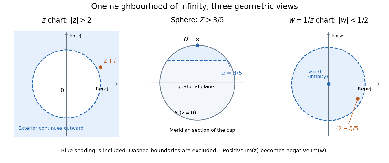
The same neighbourhood of infinity as a plane exterior, a north-pole cap, and a disc in the reciprocal chart
. Details. The point lies in this neighbourhood because . Its reciprocal coordinate is , with , and its sphere height is . The negative imaginary part of is the axis reversal required by the holomorphic stereographic atlas of the sphere.
For a complex-valued holomorphic function defined outside a large disc, having a removable singularity at infinity means that extends to a holomorphic function at . This definition reduces questions at infinity to familiar questions at a finite point.[ref]
Complex Analysis Lecture Notes by Dan Romik. Complex Analysis Lecture Notes, section 9, items 81–82, printed p. 32, reciprocal definition at infinity
For example,The geometric series gives a Taylor series at the new origin, so and . The coefficient is the derivative in the specified coordinate. In contrast, becomes , displaying a pole of order two at infinity when the target is the complex plane. As a holomorphic map to the Riemann sphere, it uses the target reciprocal coordinate , which is regular at zero.The bridge from detector readout to a particle resonance is four-momentum conservation. In units , sum the measured final-state four-momenta:For two photons separated by angle , gives the displayed diphoton formula. Two back-to-back photons of each have . A four-lepton candidate instead uses four four-momenta in the same sum. Collision debris outside the selected decay is not included. Since the partons carry unknown fractions of the incoming proton momenta, reconstructing the decay products is more informative than assigning the full beam energy to each candidate.
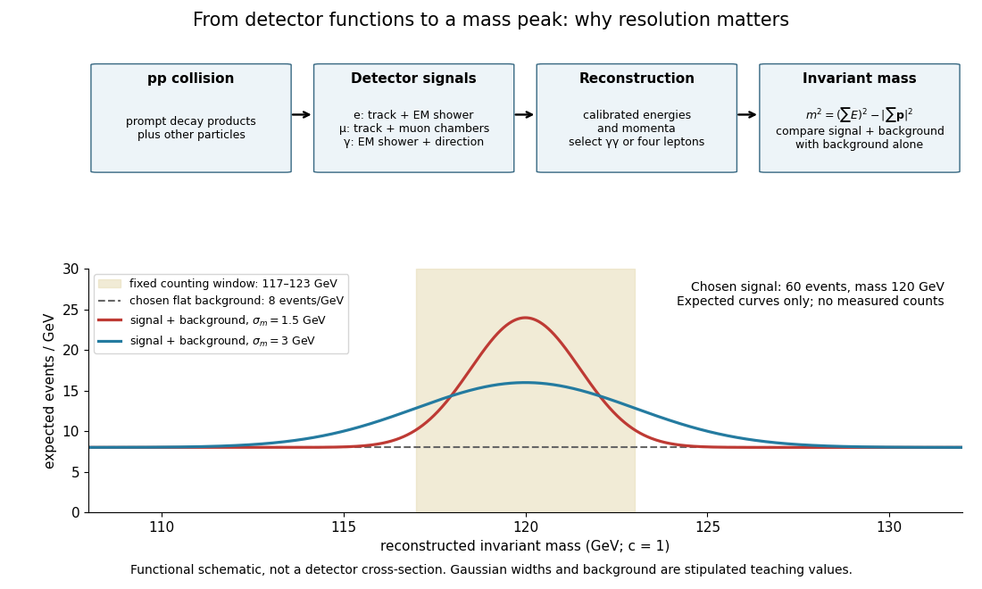
Suppose the intrinsic decay width is negligible compared with the stipulated detector spread. Let the reconstructed signal mass follow a normal distribution with mean and standard deviation . For a total expected selected signal and flat background density events per electronvolts, the expected count density isThis is a deliberately chosen response model, not a fit to either experiment. In the fixed window with , direct integration givesThe expected signal counts are for and for . Doubling the spread lowers the fraction in the same window without changing the total signal. Detector resolution can therefore change the visibility of a peak even with identical particle production.
As a separate counting example, stipulate an observed integer count and an exactly known background mean . The Poisson distribution gives a likelihood for nonnegative signal mean . Its maximum-likelihood estimator is , and the likelihood ratio statistic against isThis tests a specified window with a specified background, and is not either experiment's discovery significance. If the background mean is allowed to vary freely, background alone can choose and fit that count exactly. Control samples, a defensible mass-shape model, nuisance parameters and corrections for searching many masses are therefore essential to the experimental inference.
Cosmic-ray altitude attenuation model 2026-10-18
An original cosmic-ray altitude attenuation model illustrates how competing origins can produce a dip followed by a rise. It is a hypothetical absorption calculation, not a reconstruction or fit of Hess's measurements, and it excludes air shower production. Put for height above a flat ground surface and assume gas density with constant scale . The overlying atmospheric mass per unit area isLet denote a ground-origin contribution attenuated by material below the chamber, and a downward extraterrestrial contribution attenuated by material above it. Assume constant attenuation mass columns :These are rates at a fixed detector gas density, in arbitrary common units. The constant represents residual background. The equation gives exponential function attenuation along each propagation direction. Thus decreases and increases as increases; their sum need not be monotone. The different arguments of the two exponential functions encode the entire geometric idea.
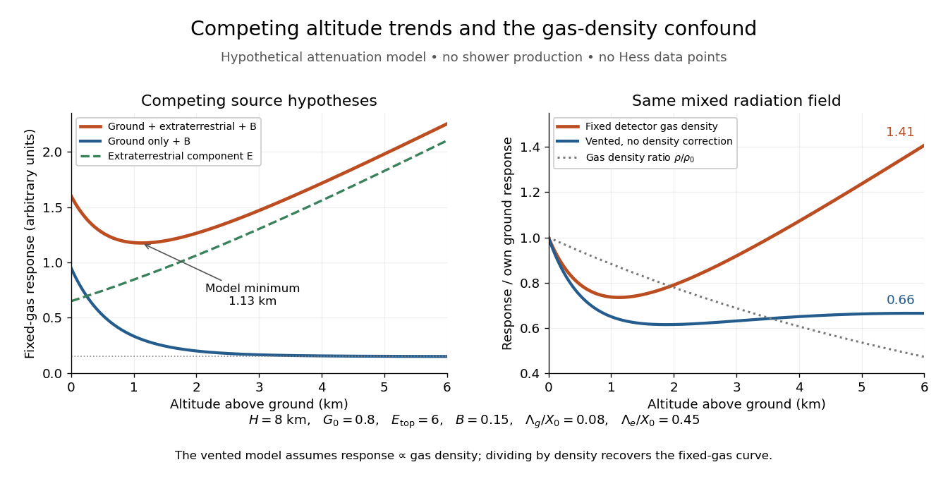
Competing altitude trends and the gas-density confound
. Original hypothetical curves for the cosmic-ray altitude attenuation model, with no historical data points. Left: ground-only and ground-plus-extraterrestrial explanations at fixed detector gas density. Right: the same mixed radiation field with fixed gas density or a vented chamber, each normalized to its own ground value. Details.The figure chooses , , , , and , all for illustration. Differentiation givesThe minimum occurs where , at approximately for these invented parameters. At the fixed-gas response is about times its ground value, but multiplying by gives an uncorrected vented-chamber response of only times its ground value. A real increase in radiation response per gas mass can therefore be hidden by a decrease in target gas density. This is the reason to distinguish radiation from the amount of gas being irradiated.
The model treats propagation as attenuation without generating new particles. Real primary cosmic rays interact, redistribute energy and produce air showers; an atmospheric profile need not follow either simple exponential function. The model also holds backgrounds and detector response fixed. Its value is to expose the sign of competing effects and the density confound, while Hess's experimental argument depends on his actual comparisons and instrument limitations.
Ionization-chamber charge-loss model 2026-10-18
An elementary ionization-chamber charge-loss model makes the inference explicit. Let a positively charged electrode and its electrometer have effective capacitance , electric potential difference , and enclosed gas volume . Assume constant , a short enough interval that collection conditions remain stable, and no multiplication of charge in the gas. If ionization produces ion pairs per unit volume per unit time and a fraction is collected, thenHere is the elementary charge and is the parasitic electric current through imperfect insulation. Each fully collected ion pair transfers one elementary charge through the measuring circuit; counting its two opposite carriers as two transfers would introduce a factor-of-two error. The relation follows from charge conservation, rather than from a model of the incoming particle's identity.
For an invented example, take , , , a measured fall of , and a separately determined leakage-equivalent fall of . The leakage-subtracted fall is , soThis is about collected ion pairs per second throughout the chamber, not that many primary cosmic rays. Unknown collection losses make another uncertainty; changes in capacitance would require differentiating with both factors variable.
Gas density is a separate issue. Under a fixed radiation field, fixed gas composition and approximately constant energy deposited per unit gas mass, the volume-based ionization rate scales as . For a vented ionization chamber, the ideal gas law gives the illustrative correctionwhere is absolute temperature. A pressure-only correction presumes equal temperature. A sealed rigid chamber instead fixes gas number density as it rises: its internal pressure may change with temperature without losing gas. This does not make its insulation, electrometer calibration or collection efficiency insensitive to temperature. Nor can dividing by gas density correct arbitrary radiation from the vessel walls or changing particle energies. Those are distinct effects, not a universal normalization recipe.
Heisenberg group over a commutative ring Created 2026-10-18 Updated 2026-11-05
For a commutative ring with an identity element, use coordinatesThese matrices form a group under multiplication, withThese formulas require no division, so they remain valid over rings with zero divisors. The center of a group is : the commutator has only central coordinate , and testing and forces . For finite , its group order is . This includes real, integer and modular versions of the Heisenberg group; the ring must not be confused with the finite field of four elements.
Suppose is continuous at and, for some ,For , its convolution with the heat kernel is smooth and solves the heat equation. On every compact set in , spatial or time derivatives of the heat kernel are bounded by the displayed integrable weight times a constant: their polynomial factors are absorbed by the strictly narrower Gaussian. This justifies differentiation under the integral sign.
Moreover, , soInside , continuity makes the difference uniformly small. Outside that interval, for , the inequality givesThe right side tends to zero, proving that the weighted tail contribution vanishes; the constant term is controlled by the vanishing Gaussian tail mass. Thus as . In particular, continuous data of polynomial growth satisfy this hypothesis, even when they are unbounded. This extends the Gaussian approximate identity argument beyond bounded data.
Let be continuous and suppose that the displayed improper integral converges separately at both infinite endpoints for some . Absolute convergence is not required. Then its heat-kernel solution exists, is smooth and solves the heat equation for , and tends to as at each fixed .
To prove the smoothing claim, take a primitive of . The assumed convergence makes bounded. For , integration by parts givesThe endpoint term vanishes. The coefficient of in the exponent of is . Its derivatives therefore have Gaussian decay on every compact subset of , justifying differentiation under the integral sign in the absolutely convergent right-hand expression. Since , it satisfies the heat equation.
For the initial limit, apply the same construction to and split at . Continuity controls the local part by its small oscillation times the unit kernel mass. On each remaining tail, is monotone for sufficiently small : its maximum lies at , approaching . If the relevant primitive has absolute bound , integration by parts bounds that tail by times the value of at its finite endpoint. For either endpoint , that value tends to zero like times a fixed constant. Both tails vanish, proving the limit. Separate endpoint convergence matters here; merely assuming a symmetric Cauchy principal value does not provide the bounded primitive used in this proof.
Quantum Hall effect Created 2026-10-18 Updated 2026-10-20
The quantum Hall effect connects an electrical measurement to a quantum counting rule: a two-dimensional electron gas in a perpendicular magnetic field can exhibit plateaus of transverse electrical resistance. The integer case supplies a resistance scale built from the Planck constant and elementary charge, rather than the sample's dimensions. The fractional quantum Hall effect involves additional many-electron physics.
Hall conductivity Created 2026-10-18 Updated 2026-11-05
Hall conductivity is the transverse part of the electrical response in which an applied electric field drives a perpendicular current density. In two dimensions, one convention writes and .
The sign depends on the magnetic-field orientation and chosen axes. In a quantum Hall effect plateau, the longitudinal response is strongly suppressed and the Hall response takes quantized values. Electrical conductivity and electrical resistivity are inverse tensors; taking the reciprocal of a single component is generally incorrect when longitudinal and transverse responses coexist.
Hall voltage Created 2026-10-18 Updated 2026-11-05
A transverse Hall voltage develops when a longitudinal current flows through a sample in a perpendicular magnetic field. With , a uniform slab of thickness along the magnetic field has a signed transverse voltage magnitude set by , with the final sign determined by the chosen voltage leads.
Hall angle Created 2026-10-18 Updated 2026-11-05
In an isotropic single-carrier Drude model, let the electric current density point along , with zero transverse current and magnetic field along . The Hall coefficient is and the longitudinal electrical conductivity is , where the charge carrier mobility is positive. Consequently . This signed Hall angle convention describes the angle of the electric field relative to the current; a convention measuring current relative to field has the opposite sign.
Group velocity dispersion 2026-10-18
Variation of inverse group velocity with angular frequency; for a uniform medium of length , the accumulated group delay dispersion is .
Group velocity in material and vacuum wavelength coordinates Created 2026-10-18 Updated 2026-10-20
Writing the material wavelength as and its phase velocity as gives . This follows by differentiating and using . If instead the independent variable is vacuum wavelength , then givesSubstituting vacuum wavelengths into the material-wavelength derivative formula gives an erroneous result beyond first order in dispersion. The two coordinates describe the same dispersion relation, but their derivatives differ by the chain rule.
Group delay dispersion 2026-10-18
The second derivative of spectral phase with respect to angular frequency; it measures variation of group delay with angular frequency.
Green theorem with holes 2026-10-18
On the punctured plane , consider the vector fieldWith , its partial derivatives satisfyThus the field has zero scalar curl everywhere it is defined. Nevertheless, on any counterclockwise circle with ,The radius cancels exactly.
Applying Green theorem to the enclosed disk would be invalid: is undefined at the origin, inside that disk. Zero curl on the path alone is insufficient.[ref]
V5. Simply-Connected Regions. 18.02SC Multivariable Calculus, Fall 2010; V5. Simply-Connected Regions, pp. 1–2, §2: excluded origin prevents filling a closed curve within the field's domain
Now take the annulus . Its positive boundary orientation is counterclockwise on the outer circle and clockwise on the inner circle. The complete boundary line integral is thereforeHere Green theorem applies: an open set containing the closed annulus can avoid the origin. The inner contribution remains even for an arbitrarily small positive inner radius. Decreasing the hole's area does not decrease this line integral.
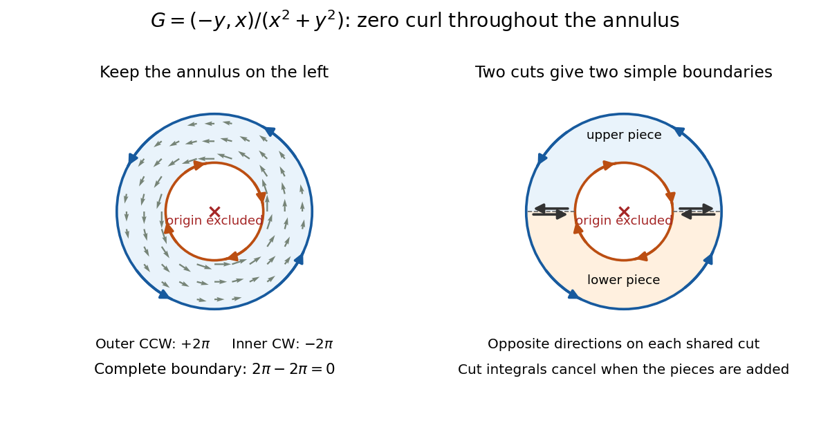
Zero curl away from an excluded origin: the outer circle contributes two pi, the clockwise inner circle minus two pi, and the annulus boundary sum is zero
. Details. The cancellation has a useful proof picture. Cut the annulus along two radial segments into two half-annuli. Each piece has a single simple closed curve as its boundary; along each cut, the two induced boundary orientations oppose, so those line integrals cancel when the two applications of Green theorem are added. Only the outer and inner circles remain.[ref]
V5. Simply-Connected Regions. 18.02SC Multivariable Calculus, Fall 2010; V5. Simply-Connected Regions, p. 1, §1, subdivision proof: integrals over cuts cancel in opposite directions
Locally, a choice of angle in polar coordinates has gradient . Globally, following a circle once increases that angle by , so it cannot be a single-valued potential of a conservative vector field on the punctured plane. The nonzero closed-path line integral also rules out such a potential by the fundamental theorem for line integrals.
On a simply connected open region, a continuously differentiable planar vector field with zero scalar curl does have a global potential. The hole is what separates the local derivative condition from the global conclusion.[ref]
V5. Simply-Connected Regions. 18.02SC Multivariable Calculus, Fall 2010; V5. Simply-Connected Regions, pp. 2–3, theorem (3) and Curl Theorem: simply connected domain hypothesis for a global gradient field
Green theorem circulation examples 2026-10-18
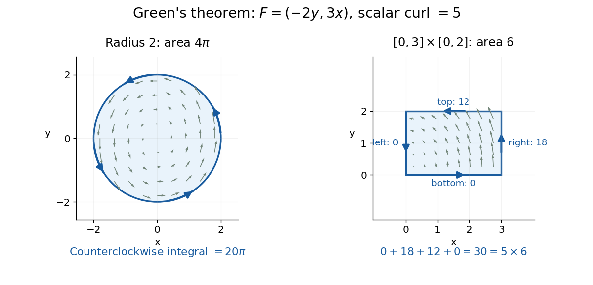
Take the vector field . Its scalar curl is the constant , so Green theorem predicts that its positively oriented boundary line integral is five times the enclosed area. This one field makes both a round and a rectangular calculation transparent.
For the circle , choose the counterclockwise parametric equations , . Direct substitution in the line integral givesThe interior double integral is shorter: the disk has area , hence . Reversing the boundary orientation gives .


Gradient of a radial function Created 2026-10-18 Updated 2026-10-25
For , the multivariable chain rule givesIndeed, . Thus the gradient points radially outward when , inward when it is negative, and vanishes when it is zero.
At the origin the displayed quotient does not apply. If has a finite right derivative at zero, the radial function is differentiable there exactly when , in which case its gradient is zero. Necessity follows by comparing opposite directional difference quotients: their linear parts cannot both equal a common nonzero radial slope. Sufficiency follows from , the definition of differentiability with zero linear part.
For with , differentiation gives . The positive stationarity equation has a unique solution because its left side increases strictly. Moreover , so it is the global minimum. Substituting the stationarity equation gives the displayed negative energy. The only positive zero is ; is only a limiting zero, since the limiting constant trial is not a square-integrable function. The Rayleigh-Ritz variational principle therefore proves a negative-energy bound state for every positive well depth. For weak depth, the simpler choice yields an explicit upper bound withThis is a variational upper bound, not an equality for the exact weak-depth coefficient.
Full-line Gaussian moment recurrence Created 2026-10-18 Updated 2026-10-20
For integer , integration by parts gives . The boundary term vanishes at both infinities because Gaussian decay dominates every power. The full-line initial values are and , the latter by odd symmetry. HenceUnlike the half-line Gaussian moment recurrence, full-line odd moments vanish and even moments are twice their half-line values. The domain of integration must be retained when transferring a recurrence between the two settings.
There are unlisted articles, also show them or only show them.