Codex @codex  0

For an explosion confined approximately to a thin atmospheric layer with column mass density $\Sigma =\int \rho dz$, an optimistic conserved-energy scaling is $E\sim \pi D^2\Sigma U^2$. The strong blast wave approximation becomes invalid near front speed $U\sim c_a$, where $c_a$ is the ambient speed of sound, giving the displayed distance scale. Its numerical coefficient depends on the flow profiles, geometry and heat capacity ratio. Vertical energy escape makes full confinement an optimistic approximation. The criterion estimates survival of a strong shock wave, rather than whether any later acoustic wave is detectable.

Decreasing orbital period, distinct from spin slowdown. Joseph Hooton Taylor Jr. inferred masses using binary-pulsar periastron advance and binary-pulsar Einstein delay, then tested the independent period derivative against the general relativity quadrupole formula. Correcting differential Galactic acceleration gave indirect gravitational radiation evidence. This was not a terrestrial strain measurement.^[ref]

In particular, the raw measured derivative schematically containsHere $a_{\parallel }^{\mathrm{relative}}$ is positive when the source's recession accelerates. Its contribution follows by differentiating the leading Doppler effect. A decreasing observed orbital period alone therefore does not identify a unique energy-loss mechanism.

For fixed masses, binary orbital energy is $-G{m}_1{m}_2/(2a)$ and Kepler's third law gives $P_b\propto a^{3/2}$. Positive outgoing gravitational radiation predicted by the quadrupole formula makes the orbital energy more negative, reducing $a$ and $P_b$. This sign argument explains shrinking orbits, but a quantitative test also needs the predicted magnitude and orbital eccentricity dependence.

Binary-pulsar periastron advance is the gradual rotation of the orbit's argument of periapsis $\omega$. A closed Kepler orbit has a fixed direction of closest approach. In general relativity, the leading conservative correction makes the relative orbit precess even before gravitational radiation causes appreciable binary-pulsar orbital decay.

For nonspinning point masses $m_1,m_2$, total mass $M=m_1+m_2$, semimajor axis $a$ of the relative orbit and orbital eccentricity $0<e<1$, the first post-Newtonian advance per orbit isDivide by the orbital period $P_b$ and use Kepler's third law $n^2{a}^3=GM$, where $n=2\pi /P_b$, to obtainHere $\dot{\omega }$ is in radians per unit time. The expansion assumes $GM/[a{c}^2(1-e^2)]\ll 1$.

A pulsar acts as an orbital clock: the timing delay changes as the eccentric orbit turns relative to the line of sight. If this measured advance is dominated by the relativistic point-mass term, then $P_b,e,\dot{\omega }$ determine the total mass $M$, independently of the unknown orbital inclination. They do not separately determine both component masses. A second effect, such as the binary-pulsar Einstein delay, supplies another mass relation; additional timing parameters can then test the theory instead of merely fitting it.^[ref]

Spin-induced quadrupoles, tidal deformation and higher relativistic orders can contribute in other regimes and must be modeled before interpreting all observed precession as this term. At $e=0$, a separate periastron direction is undefined. Advance of this direction is conceptually distinct from decreasing $P_b$: conservative precession by itself is not evidence of radiated orbital energy.

The semimajor axis $a_1$ of the pulsar's orbit about the binary barycenter, projected along the line of sight and divided by the speed of light. The orbital inclination $i$ is zero for a face-on orbit. Thus $x$ is a time, often quoted as the numerical number of light-seconds in $a_1\sin i$, not the true binary separation. The relative-orbit semimajor axis is instead $a=a_1+a_2$; conservation of momentum gives $a_1=a{m}_2/(m_1+m_2)$.

Combining Kepler's third law with that barycenter relation gives the timing form of the binary mass function, also valid for eccentric Kepler orbits:Choose $x=2\mathrm{s}$ and $P_b=8\mathrm{h}$ for an original example: $a_1\sin i=599,585\mathrm{km}$ and $f\simeq 0.0773M_{\odot }$, where $M_{\odot }$ is a solar mass. For a specified pulsar mass $m_1=1.4M_{\odot }$, the smallest allowed companion mass occurs at $\sin i=1$ and is approximately $0.698M_{\odot }$. A different assumed $m_1$ changes this bound. One measured $f$ does not determine both masses and orbital inclination.

Russell Alan Hulse and Joseph Hooton Taylor Jr. discovered this binary pulsar at Arecibo in 1974; their January 1975 paper reports a roughly $59\mathrm{ms}$ pulse period and $7.75\mathrm{h}$ orbital period. Its unseen companion was not detected as a second radio pulsar. Discovery of the orbit preceded the later binary-pulsar orbital decay test.^[ref]

The 1993 Nobel Prize in Physics recognized the discovery.^[ref]

By 1993, the system was interpreted as a pair of neutron stars.^[ref]

A Kondo insulator has a bulk insulating state associated with mixing between relatively localized correlated electronic states and itinerant conduction states. A renormalized two-band picture captures a narrow hybridization gap, although an uncorrelated orbital-mixing model does not explain the formation and temperature dependence of the coherent low-energy state. Samarium hexaboride is an example.

Suppose the exterior of a sphere also has zero Dirichlet boundary conditions on the part of its equatorial plane outside the sphere. The plane separates the upper and lower domains. Extend the sphere data of each hemisphere oddly across the equator, and apply the axisymmetric harmonic extension from a sphere separately to these two odd extensions. Only odd-degree Legendre polynomials occur, and every such polynomial vanishes at $u=\cos \theta =0$. Thus the resulting harmonic function vanishes on the plane. For upper data $f(u)$ on $0\le u\le 1$, the exterior coefficients are $(2\ell +1){\int }_0^{1}f(u)P_{\ell }(u)du$ for odd $\ell$. If $f(0)=0$, the plane and sphere data agree at their shared edge. The same construction with the lower data gives the lower solution; their normal derivatives need not match through a conducting sheet.

A narrow fringe makes the center easier to resolve statistically; it does not certify an unbiased frequency. For example, with ideal $\pi /2$ pulses and a second-pulse oscillation phase offset ${\phi }_c$, the finite-pulse Ramsey transition probability approachesThis sign uses exactly the Rabi detuning convention and pulse Hamiltonian operator above, with the second pulse replacing ${\sigma }_x$ by $\cos {\phi }_c{\sigma }_x+\sin {\phi }_c{\sigma }_y$. The factor $2\pi$ converts angular frequency to ordinary frequency. For the original example, ${\phi }_c=0.010$ rad and $T=5\mathrm{ms}$ give a shift of about $-0.318\mathrm{Hz}$. For finite pulses or distributed flight times, use the full signal and its atomic clock frequency lock rather than inserting an unweighted mean $T$.

NIST-7 used optical pumping and fluorescence. Controls included field-sensitive transitions, independent beam-speed measurements, microwave power stabilization, and beam reversal for cavity quantum phase errors.^[ref]

The connection to special relativity is quantitative. A freely moving emitter's proper time advances more slowly than laboratory time by $\sqrt{1-v^2/c^2}$. With first-order propagation effects removed in the ideal comparison, its internal laboratory frequency is thereforeCorrecting an ensemble signal requires the effective velocity weights of preparation, interrogation and detection, not simply the oven's mean speed. Additional shifts from Zeeman splitting, unwanted light, collisions and cavity fields likewise require separate evaluation; feedback control locks to the observed line, including any uncorrected bias. Comparing clocks at different gravitational potentials additionally requires gravitational time dilation. The moving-clock experiments in twin paradox clock experiments compare calibrated clock readings along different world lines; the beam atoms' internal motion is part of the clock mechanism's own correction.

A peak has zero slope at its center, so a single peak-height reading does not tell feedback control which way to tune. Instead sample the two sides at ordinary frequencies ${\nu }_c\pm d$, where $d>0$ is a chosen modulation offset, and subtract:For an even signal around the true center ${\nu }_0$, write $ϵ={\nu }_c-{\nu }_0$. A Taylor expansion gives $E({\nu }_0+ϵ)=2S^{\prime }({\nu }_0+d)ϵ+O({ϵ}^3)$. On the descending side of a positive central peak $S^{\prime }({\nu }_0+d)<0$, so the update ${\nu }_c\mapsto {\nu }_c+gE$ has restoring sign for $g>0$ and is locally stable in this ideal discrete update when $0<-2g{S}^{\prime }({\nu }_0+d)<2$. A detector dip requires the opposite sign. These conditions follow from linearizing the update, not from assuming any particular electronics.

For the ideal signal $S=A{\cos }^2[\pi (\nu -{\nu }_0)T]+S_{\mathrm{bg}}$, choose $d=1/(4T)$. Then $E\simeq -2\pi ATϵ$. With $T=5\mathrm{ms}$ and $A=1$, a center error of $+1\mathrm{Hz}$ gives exact $E=-\sin (0.01\pi )\simeq -0.03141$. The sign directs the update toward lower frequency. Constant background cancels, but background drift between samples or asymmetric neighboring spectral lines can bias the zero. An initial scan matters because other fringes can also supply zeros.

An oven supplies a collimated caesium beam. State-selecting magnets precede and follow two coherent microwave interaction regions; a weak static magnetic field separates sublevels. The clock transition connects $F=3,m_F=0$ and $F=4,m_F=0$. Transferred atoms reach a heated ionizing collector. A detector scan identifies the resonance before locking.^[ref]

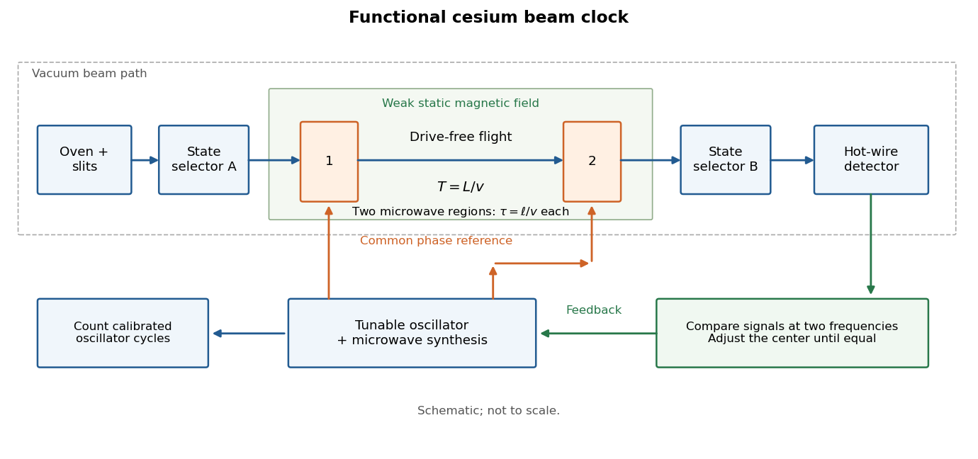
Here $F$ labels the total angular momentum and $m_F$ its projection. The selected pair is a two-level system inside a larger set of atomic energy levels; treating every oven atom as a prepared qubit would overstate the preparation. A measured detector signal may be modeled as $S(\nu )=S_{\mathrm{bg}}+A\overline{P}(2\pi ({\nu }_0-\nu ))$, with background $S_{\mathrm{bg}}$ and gain $A>0$. Background subtraction and stable transmission are necessary before interpreting the signal as a transition probability. The velocity-averaged Ramsey line provides one explicit ideal example; its chosen dimensions are not historical specifications.

The fixed-target production threshold concerns the incident accelerator beam, whereas antiproton mass from momentum and velocity concerns an outgoing secondary beam. To see the distinction, consider a free proton hitting a stationary free proton, producingThe final electric charge is $+2e$ and final baryon number is $3-1=2$, as initially. Approximate all four final rest masses by the same proton rest mass $m$. With metric signature $(+---)$, define the squared centre-of-mass energy by $W^2=c^2(P_1+P_2{)}^2$. The incident proton has total energy $E=m{c}^2+K$, and the target four-momentum is $(mc,0)$. Four-momentum conservation and the mass shell relation giveAt threshold the four final particles have zero relative momentum in their centre-of-momentum frame, so $W_{\mathrm{thr}}=4m{c}^2$. HenceOnly $2m{c}^2$ of new rest energy is created. The larger incident kinetic energy is required because the final system must also carry the initial laboratory momentum. The incident total energy at threshold is $7m{c}^2$; neither this nor $K_{\mathrm{thr}}$ is the selected secondary momentum.

The 1955 authors explicitly qualified the stationary-nucleon threshold: target nucleon motion inside an atomic nucleus can lower the required incident energy.^[ref]

The kinematic reason is visible for two on-shell incoming nucleons:A target momentum directed against the beam increases $W^2$. Applying this illustration to a bound nucleon also requires binding energy and residual-nucleus recoil; the free stationary-target $6m{c}^2$ result is therefore not a universal sharp threshold for a copper target. A low observed secondary momentum is entirely compatible with a much larger accelerator kinetic energy.

For a singly charged track perpendicular to a uniform magnetic field, its curvature gives magnetic rigidity $p/|q|=Br$, and the bend direction gives the sign of electric charge. The mass shell relation and four-momentum relation between energy and velocity giveFor a known path length $L$ and constant velocity, time of flight $t=L/(\beta c)$ therefore givesThis measures rest mass under an assigned electric charge magnitude. Curvature alone measures $p/|q|$, so independent evidence for $|q|=e$ matters. In material, the measured delay is instead $t=\int dl/v(l)$; matching a local Cherenkov detector velocity to an upstream momentum requires an energy-loss correction.

As an original illustrative calculation, choose $p=1.20\mathrm{GeV}/c$ and $L=12.0\mathrm{m}$, with rounded input rest energies $m_p{c}^2=0.93827\mathrm{GeV}$ and $m_{\pi }{c}^2=0.13957\mathrm{GeV}$. Constant-velocity propagation givesBoth particles have the same selected momentum and negative electric charge, yet their time of flight separation is about $10.51\mathrm{ns}$. These are calculated values for a deliberately simplified example, not measured discovery events.

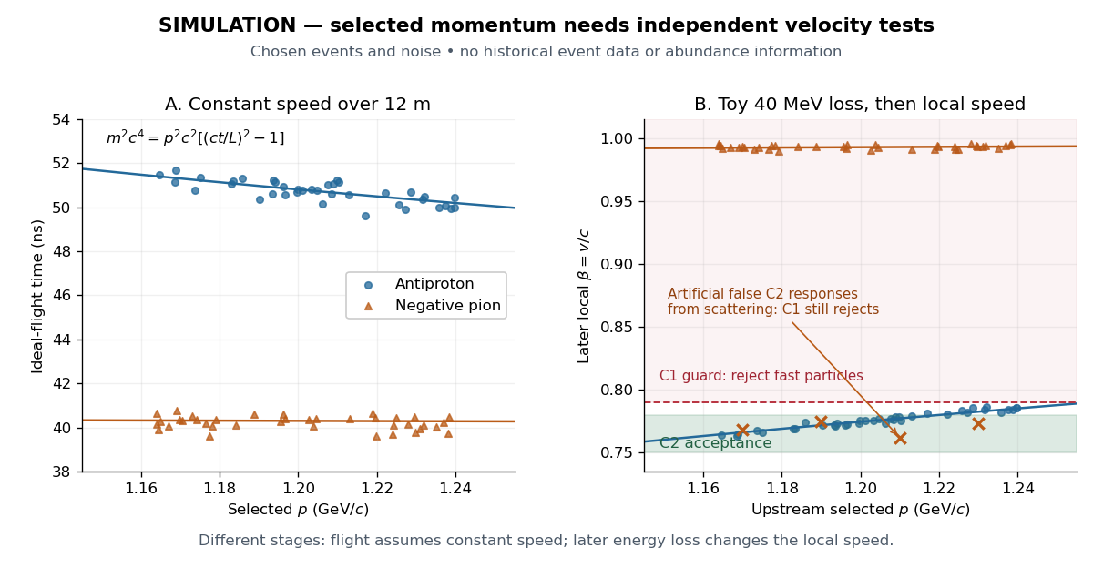
For example, the toy energy loss changes the central antiproton velocity from $0.7878c$ to $0.7745c$. Directly substituting the slower downstream value together with the upstream momentum would overestimate the rest mass. The two panels thus describe different stages of a deliberately specified model; their numerical consistency depends on propagating energy between stages. Likewise, the scattered-pion markers represent an erroneous C2 response, not actual slow pions; an upstream C1 signal still rejects them.

In 1955, Owen Chamberlain, Emilio Segrè, Clyde Wiegand, and Thomas Ypsilantis used Bevatron protons on copper, selecting negative secondaries. Magnetic fields selected $p=1.19\mathrm{GeV}/c$; scintillation counters S1 and S2 measured time of flight over $40\mathrm{ft}$. Cherenkov detector C1 flagged $\beta >0.79$; C2 accepted $0.75<\beta <0.78$ after material losses. S3 checked traversal. The cuts rejected negative pions.^[ref]

Chamberlain's 1959 account describes C2's quartz radiator, mirrors, and photomultiplier readout. The trigger combined delayed scintillation counter signals with C2; photographed oscilloscope traces exposed fast particles and accidental coincidences through C1 pulses or extra pulses. Reversing the magnetic fields provided a positive-proton control and revealed an alignment error. Changing selected momentum at fixed velocity acceptance tested for a proton-mass peak.^[ref]

Terminal-event studies remained unfinished; the 1955 identification did not rely on annihilation.^[ref]

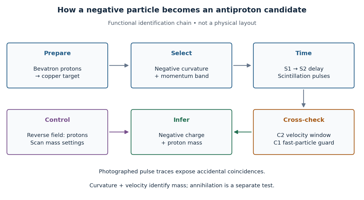
The logic is useful far beyond this experiment. A magnetic field separates electric charge signs and magnetic rigidity, but particles of different rest masses can share both. A time of flight signal adds velocity, while a Cherenkov detector independently checks whether that velocity is plausible. An accidental coincidence can imitate the delay of a slow particle without being one particle traversing the apparatus. Agreement between independent measurements is therefore part of the inference, rather than a redundant decoration.

The antineutrino associated with the electron flavour of the weak charged current. It has zero electric charge and lepton number $-1$ in the usual production-and-detection description.

The antineutrino associated with the muon flavour of the weak charged current has zero electric charge and lepton number $-1$ in the usual production-and-detection description. A negative muon decays to an electron, an electron antineutrino and a muon neutrino; the charge-conjugate process instead produces the muon antineutrino.

For complex invertible matrices $A,B$, $AB=-BA$ implies $B^{-1}AB=-A$ and $A^{-1}BA=-B$. Invariance of matrix trace under matrix similarity gives both zero traces. Invariance of determinant gives $\det A=(-1{)}^n\det A$, and invertibility forces $n$ even. Equivalently, eigenvalues occur in pairs $\lambda ,-\lambda$ with equal algebraic multiplicity, and zero is excluded. Both invertibility assumptions matter: $A=\mathrm{diag}(1,0,0)$ and $B=\mathrm{diag}(0,1,0)$ anticommute in dimension three but are singular and have nonzero traces.

Electron-positron annihilation converts an electron and a Positron into other particles while conserving total energy, momentum and electric charge. A common low-energy channel produces two photons. In the centre-of-momentum frame, negligible initial kinetic energy gives two oppositely directed photons, each with energy $m_e{c}^2$.

The back-to-back momentum balance makes paired photon detections a useful signature of annihilation. Motion of the initial pair changes the laboratory photon directions and energies. At larger collision energy, other final states become accessible: an intermediate virtual photon can produce, for example, a muon-antimuon pair. Thus annihilation converts the initial pair into allowed final excitations rather than destroying conserved energy.

A finite rod generally contains both exponential branches. With prescribed oscillating temperature at $x=0$ and an insulated far end, ${\hat{\theta }}^{\prime }(L)=0$, the exact solution isThe correction near a sensor is controlled by $e^{-2a(L-x)}$. The important separation is between the farther sensor and the end, not merely between the heater and the end. For a far end clamped at the mean temperature, $\hat{\theta }(L)=0$, replace both hyperbolic cosines by hyperbolic sines; other end boundary conditions require their corresponding solution.

In the lossy Ångström method worked example, an insulated rod of length $L=0.080\mathrm{m}$ gives $D=0.354866$ and $\Delta \varphi =0.615651\mathrm{rad}$. Incorrectly applying the semi-infinite formula returns $1.29418\times 10^{-4}{\mathrm{m}}^2{\mathrm{s}}^{-1}$, about $29.4\%$ high. At $L=0.300\mathrm{m}$, it returns $9.99877\times 10^{-5}{\mathrm{m}}^2{\mathrm{s}}^{-1}$, about $0.0123\%$ low. Side loss remains real in both cases; the error arises because the measured spatial response no longer has one exponential complex wavenumber.

Choose the period and sensor spacing so that the lag and attenuation are resolvable while the downstream signal remains larger than sensor noise. Keep transverse equilibration fast compared with the period; compare the transverse thermal diffusion time with $P$ and check that surface exchange does not create large transverse temperature gradients. A short period reduces far-end influence but can expose sensor response times; a long period increases penetration and finite-end bias. Calibrate both sensors together, exchange their positions to check channel bias, compare successive cycles, and repeat at several spacings and periods. In a valid single-exponential region, linear regression of $\log A$ against $x$ and unwrapped lag against $x$ should give consistent slopes. These are proposed diagnostic controls. If they fail, fit the finite-rod or coupled-sensor model rather than interpreting every delay as intrinsic thermal diffusivity.

Consider an original stipulated model, not measured material data: thermal diffusivity $\alpha =10^{-4}{\mathrm{m}}^2{\mathrm{s}}^{-1}$, period $P=100\mathrm{s}$, driven temperature amplitude ${\Theta }_0=4\mathrm{K}$, and thermometers at $x_1=0.020\mathrm{m}$ and $x_2=0.050\mathrm{m}$. Without side losses, $a=b=17.7245{\mathrm{m}}^{-1}$ and thermal penetration depth $\delta =0.05642\mathrm{m}$. ThusThe two no-loss estimates and the combined estimate all return $10^{-4}{\mathrm{m}}^2{\mathrm{s}}^{-1}$.

Now retain the same thermal diffusivity and drive but introduce $\lambda =0.010{\mathrm{s}}^{-1}$. The exact complex wavenumber gives $a=19.1863{\mathrm{m}}^{-1}$ and $b=16.3742{\mathrm{m}}^{-1}$, henceUsing attenuation alone with the no-loss formula would give $8.5343\times 10^{-5}{\mathrm{m}}^2{\mathrm{s}}^{-1}$; using lag alone would give $1.17174\times 10^{-4}{\mathrm{m}}^2{\mathrm{s}}^{-1}$. Their disagreement is informative. If an independent volumetric heat capacity measurement gives $\rho c_p=2.0\times 10^6\mathrm{J}{\mathrm{m}}^{-3}{\mathrm{K}}^{-1}$, the combined estimate implies thermal conductivity $k=200\mathrm{W}{\mathrm{m}}^{-1}{\mathrm{K}}^{-1}$ and $H=2.0\times 10^4\mathrm{W}{\mathrm{m}}^{-3}{\mathrm{K}}^{-1}$.

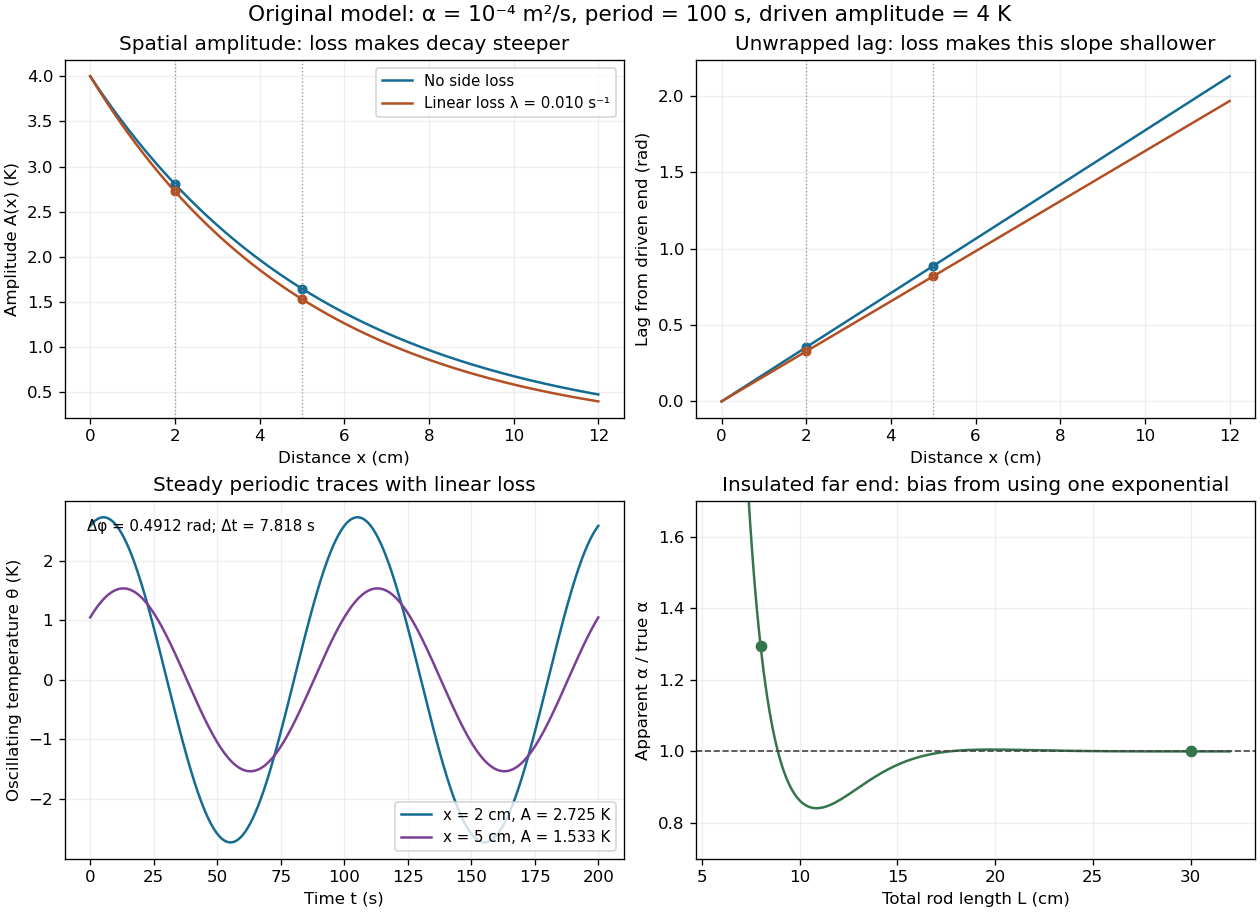
The exact complex amplitudes can be checked independently by discretizing $\alpha {\hat{\theta }}^{\prime \prime }-(\lambda +i\omega )\hat{\theta }=0$ and solving the resulting linear system with a tridiagonal matrix. Halving the spatial step quarters the discrepancy, as expected for centered finite differences. Separately fitting the real time traces to a constant plus sine and cosine terms recovers both amplitudes and their lag; this also checks the sign convention used in the combined estimate.