
Gaussian initial data for the heat equation 2026-10-18
For , the displayed function solves the heat equation and has initial condition . Set . Direct differentiation givesThese identities prove the equation. The total integral is , independent of time. The real smooth formula is valid for , including a finite interval of negative time for this particular initial profile. For nonzero , its value at diverges as the lower time endpoint is approached. The superposition principle combines finitely many such profiles with different centers or widths.
For the Gauss-Seidel iteration for a two-variable positive-definite system, define the forward error by and . Subtract the two exact solution equations from the two update equations:The fresh first coordinate passes the old second-coordinate error through two successive factors. The iteration matrix is thereforeIts eigenvalues are and , as seen from the determinant. The zero eigenvalue explains why the old first-coordinate error disappears completely: the first row overwrites it. After one sweep, every remaining forward error lies on the eigenvector line spanned by .
For this zero start, , so the exact vectors for areThe Euclidean norm of the forward error decreases by exactly per sweep from onward. The first decrease is different because the initial error has not yet reached that eigenvector line. Each row update moves horizontally or vertically in the coordinate plane; sweep endpoints then approach the solution along one straight line.
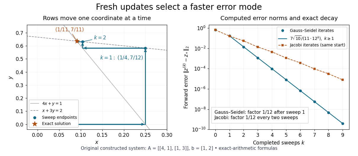
Computed row-by-row Gauss-Seidel method trajectory and exact forward error contraction for the original two-variable linear system
. Details. The linear-system residual is an independent way to check the calculation. Completing a sweep satisfies the second row exactly, but changing disturbs the first row:Thus a zero residual in the last updated row alone does not certify a solution; inspect the complete linear-system residual.
For the same matrix, the stale schedule of the Jacobi method gives the iteration matrixHere its eigenvalues are , whereas the fresh schedule gives . This comparison belongs to this particular linear system; it is not a universal relation between the two methods' spectral radii.
An invertible matrix and nonzero diagonal entries make the update well defined, but do not guarantee convergence. For the original linear systemthe Gauss-Seidel method updates and . Starting at zero gives , then . The second-coordinate forward error is , and the iteration matrix has spectral radius . The linear system has a unique solution while this particular stationary iterative method for a linear system diverges.
For a bound Kepler orbit, specific orbital energy is negative. Therefore . A projected separation and a systemic-motion-corrected line-of-sight speed give the displayed lower bound. One position and one spectral velocity already constrain the mass in this model; a fitted orbit gives much more. The bound assumes a bound orbit in a point-mass potential; it is not an unrestricted enclosed-mass formula for an arbitrary extended potential.
A chosen stellar-orbit mass estimate 2026-10-18
Choose , arcseconds, years, and degrees. The small-angle conversion gives . Taking one model year as days gives and .
Dividing by the nominal solar mass parameter, , gives nominal solar masses. The nominal parameter is an exact conversion convention, rather than an assertion that the Sun's measured mass is exact.[ref]
Resolution B3 on recommended nominal conversion constants for selected solar and planetary properties by International Astronomical Union. PDF pp.2–3, exact nominal solar mass parameter and conversion recommendation
The chosen periapsis radius is . Its corresponding Schwarzschild radius, , is about . Thus this illustrative orbit remains roughly Schwarzschild radii from the centre at closest approach. Inferring a very concentrated mass from such an orbit is different from directly resolving its event horizon. Every number here follows from the chosen orbit, not from a fit to the actual Galactic-centre measurements.
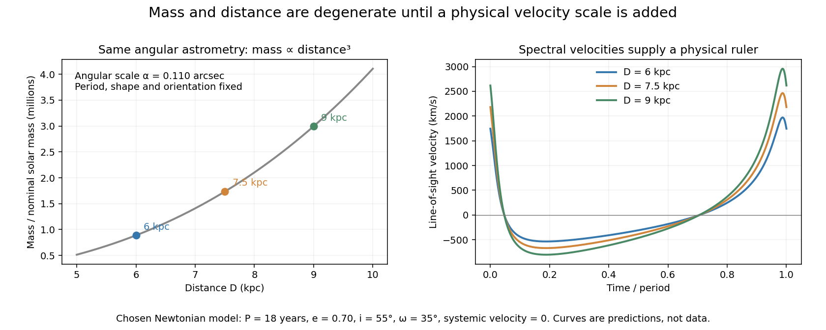
Angular astrometry determines the combination displayed by substituting into Kepler's third law. Keeping the fitted shape, orientation and orbital period fixed, the rescalingleaves the entire angular time series unchanged. A longer physical orbit around a larger mass can trace precisely the same angular path. More angular samples improve the fitted combination; by themselves they cannot break this scaling symmetry of the model.
The radial-velocity semi-amplitude isFor , combining it with the angular fit gives the orbital parallax distanceThe spectral velocity scale supplies the missing physical ruler. For a face-on orbit, , this radial signal vanishes and that method cannot supply a distance. In a partial or noisy data set, fitted orientation and systemic motion also correlate with the inferred scale.
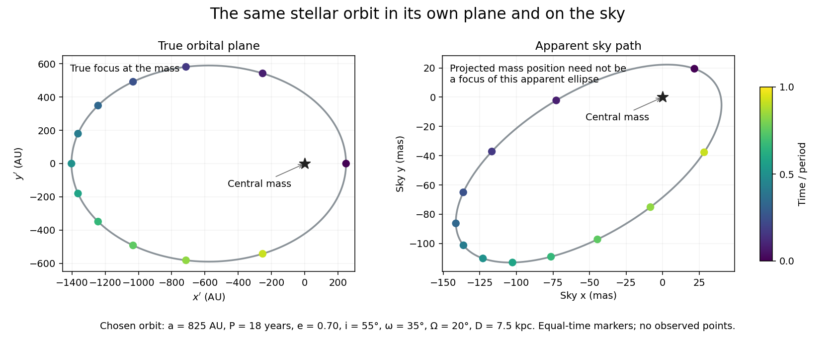
Let increase away from the observer, with spanning the sky plane. A rotation sends the orbital-plane coordinates to . Here is orbital inclination, the longitude of ascending node, and the argument of periapsis. For distance , the small-angle model gives angular positions , in radians. Doppler spectroscopy instead supplies the line-of-sight velocity , with a fitted systemic offset .
Define , the angular scale of the deprojected fitted orbit. It is not generally the semi-major axis of the apparent ellipse on the sky. Projection also need not send a true focus to a focus of the apparent ellipse. Fitting the rotated orbit preserves that distinction; measuring a bounding ellipse alone loses it.


For a complex irreducible representation of a finite group , the sum commutes with every : conjugation sends its summands to , merely permuting the summation index. Schur's lemma gives . Taking the trace yields , proving the identity. Here is the Frobenius-Schur indicator. For a reducible representation the sum is still central in its image, but need not be one scalar on all irreducible constituents.
Brewster's angle Created 2026-10-18 Updated 2026-11-05
For an interface between two lossless, isotropic, nonmagnetic media with unequal refractive index values , Brewster's angle is the incidence angle at which the reflected amplitude in transverse magnetic polarization vanishes. The Fresnel equations and Snell's law give ; the reflected and transmitted rays are perpendicular there. The usual formula assumes equal magnetic permeabilities.
For the regular isothermal Lane-Emden equation, the first fixed-mass pressure turning point occurs at . Thus the boundary radius there is , where is the squared isothermal sound speed. The approximate choice gives coefficient . Comparing with the Jeans length requires specifying the reference density and remembering that the latter is a wavelength rather than a boundary radius.
Sine eigenvectors of the fixed-end spring chain Created 2026-10-18 Updated 2026-11-05
For identical masses between fixed walls with equal springs, the dimensionless stiffness matrix has diagonal entries and adjacent entries . Its normalized eigenvectors and eigenvalues areExtend each vector by . The sine addition identity gives , including the fixed-end rows. The finite sine orthogonality identity supplies the normalization and makes distinct vectors orthogonal. The normal mode angular frequencies are for mass and spring constant . This complements the fixed-end spring-chain determinant and its repeated-root limit with the spatial mode shapes.
Three-dimensional free-electron density of states Created 2026-10-18 Updated 2026-10-20
For the uniform noninteracting electron model with two spin states and kinetic energy of nonrelativistic particles , count all available one-particle states up to an energy :This extensive density of states has units of inverse energy; is the density of states per unit volume. Availability and occupation are different: is positive above , but at zero temperature those states are empty. The occupied energy distribution is , with the Fermi-Dirac distribution reduced to below and above it. The convention at the exact boundary does not affect a continuum integral.
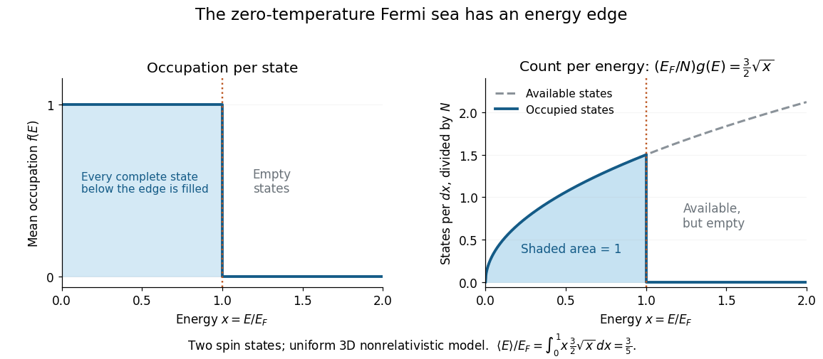
At zero temperature occupation cuts off at the Fermi energy although the density of available states keeps growing
. Details. 
With the dimensionless quantity , the occupied count per , divided by the total particle number, is for . Its area is one. Weighting this by gives the internal energy and its mean per particle:Thus the highest occupied energy and the mean energy differ. For the Fermi energy of a model electron gas, . At fixed , , so the derivative gives the electron degeneracy pressure . The same state-counting geometry therefore predicts a nonzero pressure at zero temperature.
Fermi wavevector Created 2026-10-18 Updated 2026-11-05
The Fermi wavevector is the radius of the occupied sphere in wavevector coordinates for an isotropic Fermi gas. In the uniform two-component electron model, and for nonrelativistic particles. Its units are inverse length, whereas the Fermi momentum has units of momentum.
Fermi velocity 2026-10-18
The group velocity of an excitation evaluated on the Fermi surface. For an isotropic dispersion relation , , where is the Fermi momentum.
Electron-phonon scattering Created 2026-10-18 Updated 2026-11-05
In electron-phonon scattering, an electron changes its energy by while its crystal momentum changes by a phonon wavevector modulo a reciprocal lattice vector. Charge-transport relaxation weights a scattering angle by . Small-angle events can therefore relax heat efficiently while relaxing electrical current weakly. At temperatures above the phonon excitation scale, scattering becomes approximately elastic in the electron thermal shell; residual elastic disorder often dominates at very low temperature.
Peierls transition Created 2026-10-18 Updated 2026-10-20
A Peierls transition, named for Rudolf Peierls, is a metal-insulator transition caused by a Peierls distortion of an initially metallic chain.[ref]
Peierls transition. Entry P04468: electronic transition caused by a structural distortion and opening a gap at the Fermi energy
A modulation at mixes states near opposite Fermi points and can open a band gap at the Fermi energy. At half filling with one atomic orbital per chemical atom, this modulation doubles the original lattice period and alternates strong and weak bonds. In a weak-coupling zero-temperature description, the Peierls energy gain is proportional to whereas the elastic cost is proportional to , where is the undistorted hopping strength and its small alternating change. The logarithm permits a distortion at arbitrarily weak coupling in the ideal model. Finite temperature, finite size, interchain coupling and thermal fluctuations matter for a real transition; strictly one-dimensional reasoning alone does not establish finite-temperature long-range order. Degeneracy-pressure bulk modulus Created 2026-10-18 Updated 2026-10-20
For a nonrelativistic zero-temperature free electron model with fixed particle number, electron degeneracy pressure obeys . Consequently its bulk modulus is . At temperatures small compared with the electron Fermi temperature, the leading isothermal compressibility is . This electronic contribution alone omits ionic binding and interaction corrections in a real metal.
Radiative spin-down of a rotating electric dipole Created 2026-10-18 Updated 2026-11-05
A permanent electric dipole moment of magnitude rotating perpendicular to a fixed axis emits in the electric-dipole approximation for radiation, with . For fixed mechanical moment of inertia , weak radiative loss gives and hence the displayed spin-down law. It assumes : the full dipole acceleration has squared magnitude , whose second term is beyond this leading adiabatic approximation.
Alternating-current drift excursion Created 2026-10-18 Updated 2026-10-20
For sinusoidal current density and constant carrier density , the electron drift velocity is . Its displacement has amplitude and zero net change over a full cycle. The distance accumulated by this drift alone in one cycle is . With an RMS current, . This does not measure the much larger microscopic path due to Fermi velocity and electron-phonon scattering.
Removing a singular axis in a flux integral 2026-10-18
A vector field singular on an axis need not satisfy the classical divergence theorem on the original closed region. Remove a thin tube , apply the theorem to the remaining smooth region, then examine the added cylindrical boundary. If its flux tends to zero and the remaining volume integral converges, the improper boundary flux equals the improper integral of the divergence. For with , the cylindrical unit normal has zero component, so the added flux is on a bounded axial interval. The divergence is locally integrable under the cylindrical coordinates measure . Hence no finite line-source correction survives, despite the field itself being unbounded.
There are unlisted articles, also show them or only show them.