
Polynomial flux through a half-ellipsoid 2026-10-18
For the upper curved half of , take the vector field and outward unit normal. Its divergence is . The odd term integrates to zero over the half-ellipsoid. Scaling a unit half-ball gives . The equatorial closing disk has downward flux . The divergence theorem therefore gives the displayed curved-surface flux. The constant vertical component is not detected by the divergence, but is recovered by accounting for the closing disk.
Consider the vector field in the open unit cube, where and extend to continuously differentiable functions on , and is continuous on with . Even if is unbounded as , the normal component on an -face has the finite trace . The two -faces have finite improper integral fluxes and therefore cancel. The remaining face contributions giveTo justify this use of the divergence theorem, first apply it to , on which the field is regular. Its divergence is , independent of . Its outward flux is . Taking yields the displayed answer, and absolute convergence makes the two -face limits finite separately. For example, diverges at zero butThis argument defines the normal traces and the face integrals explicitly; it does not assert that the whole vector field has a finite value on the singular face.
Conical flux by closing with a cap Created 2026-10-18 Updated 2026-10-20
To evaluate outward flux through the lateral surface of a finite right circular cone, add its planar cap and apply the divergence theorem to the enclosed solid. Subtract the cap flux, whose outward normal points away from the solid. For a cone with , the volume element is and the cap has radius . The cone's vertex has no unique normal, but is a set of area zero; one can remove a small tip and take a limit when the field is regular there.
For two planes and with linearly independent normal vectors, put , , and . Their intersection is a line parallel to . Its closest point to the origin is orthogonal to that direction, hence has the form . The constraints give , , soFor every other point , orthogonality gives squared distance , proving the global minimum and its uniqueness. The positive determinant also proves that an intersection exists for every real . Parallel normals require a separate consistency check and do not define a unique intersection line.
Two-point-source aperture synthesis 2026-10-18
Choose two point-like astronomical sources with and , where the angles are in radians and strengths use arbitrary common units. Their separation is radians. These are invented model parameters, not historical measurements. Their complex visibility follows immediately from the preceding derivation, and its squared magnitude isAt , ; at , ; at , . The unequal strengths prevent the complex visibility magnitude from reaching zero. Its modulation contains the source separation, while a common displacement of both sources changes wave phase without changing this magnitude. Amplitude alone loses that location information.
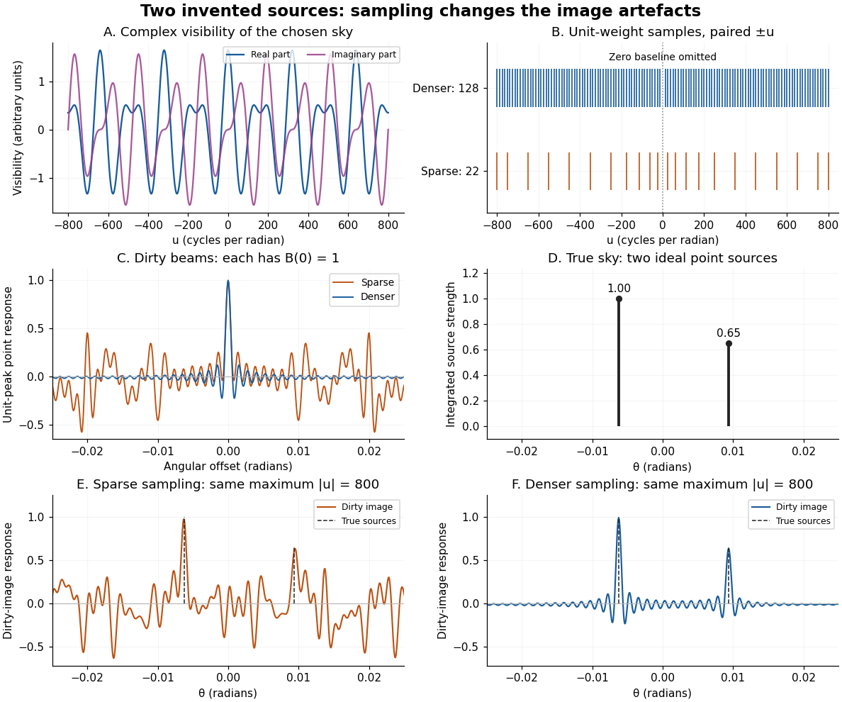
An original two-source model: complex visibility, sampling gaps, unit-peak dirty beams, and dirty images
. Details. 
The sparse case samples for ; the denser case samples every , also with both signs. All weights are one. Both reach , so their shortest fringe period is the same radians. Their dirty beams and false subsidiary features differ because the intermediate spatial frequencies differ. Neither case includes or frequencies above that maximum. The figure uses a periodic angular interval of length radians; this artificial boundary makes a discrete Fourier transform calculation exact for the chosen grid, rather than modelling an all-sky observation.
The plotted dirty image is the sum of two shifted dirty beams, not a fitted or deconvolved estimate of the source. Adding samples in this example reduces prominent spurious peaks; it does not establish a universal monotonic improvement for every weighting or sky. A missing zero baseline leaves the periodic dirty image with zero mean, so it cannot by itself recover the total positive brightness. Missing short spacings also weaken constraints on extended smooth emission.
Reconstruction is an inverse problem. A perturbation whose Fourier transform vanishes at every sampled coordinate can be added without changing the measurements: incomplete coverage leaves a null space. Nonnegative brightness, a restricted source region, or a model with a small number of components can reduce ambiguity, but each is additional information. Removing dirty beam artefacts means estimating a sky consistent with both data and such assumptions; a narrow central peak alone does not certify a unique image. Measurement error, uncertain calibration and source variability add further limitations.
Bose-Einstein condensation concerns occupation of a one-particle state. Matter-wave coherence concerns field correlations between positions or times. Superfluidity concerns a flow response, including suppression of dissipation under appropriate conditions. A density peak diagnoses neither a relative quantum phase between two separately prepared clouds nor a critical flow speed. These observables require different experiments.
For example, in a single-mode fixed-number Fock state, but . Writing for that occupied mode givesThus vanishing mean field does not imply vanishing first-order matter-wave coherence. For two independent fixed-number modes, : there is no ensemble mean interference term establishing a fixed relative quantum phase. Interpreting fringes in an individual detection record requires considering correlations and the measurement; assigning a pre-existing definite relative quantum phase is unnecessary.
Wolfgang Ketterle's lecture describes a separate coherence test: two condensates expanded into one another and produced fringes. Selectively removing one condensate made the fringes disappear on alternating preparation cycles, testing against diffraction from the confinement. This compared two-cloud and one-cloud signals; it did not measure dissipationless flow.[ref]
Nobel lecture: When atoms behave as waves: Bose-Einstein condensation and the atom laser by Wolfgang Ketterle. pp. 1143–1145, Fig. 15, condensate-elimination control
The 1995 sodium experiment combined laser cooling with a magnetic quadrupole trap and a repulsive optical plug protecting its field zero. Radio frequency evaporation preceded release and absorption imaging after time of flight. Lowering the evaporation cut produced broad thermal wings and a narrow core. Moving the plug changed the core's expansion orientation while the thermal distribution remained spherical: a control connecting the feature to confinement. Overlap of the two trapped pockets and residual switch-off acceleration limited quantitative shape comparisons; repulsive interactions affected expansion.[ref]
Bose-Einstein Condensation in a Gas of Sodium Atoms by K. B. Davis and others. pp. 3969–3972, Figs. 1–4
The rubidium experiment used laser cooling, a magneto-optical trap and magnetic trapping of neutral atoms with a rotating bias field. Radio frequency transitions removed energetic atoms; elastic collisions restored thermal equilibrium. Before absorption imaging, the trap was decompressed, then nearly released with a gradient supporting against gravity. Varying the final evaporation cut revealed a narrow anisotropic core within an isotropic thermal cloud. The broad component supplied a simultaneous comparison through the same optics. Resolution and size calibration limited inference; interactions broadened the core relative to an ideal gas.[ref]
Synthetic bimodal profile of a Bose gas 2026-10-18
A broad component plus a narrow central component can have one local maximum while still displaying two distinct width scales. This is what “bimodal” means in this imaging context; it does not require two separated peaks. To isolate the population effect, construct an original normalized line profileBoth terms are normal distributions; their integrals are one, so the component areas are and . With , the narrow component has central height , while the broad component contributes . A tall central feature therefore need not contain most of the particles. Holding these widths fixed deliberately isolates changing weights; it does not model how temperature, interactions or camera resolution determine actual widths.
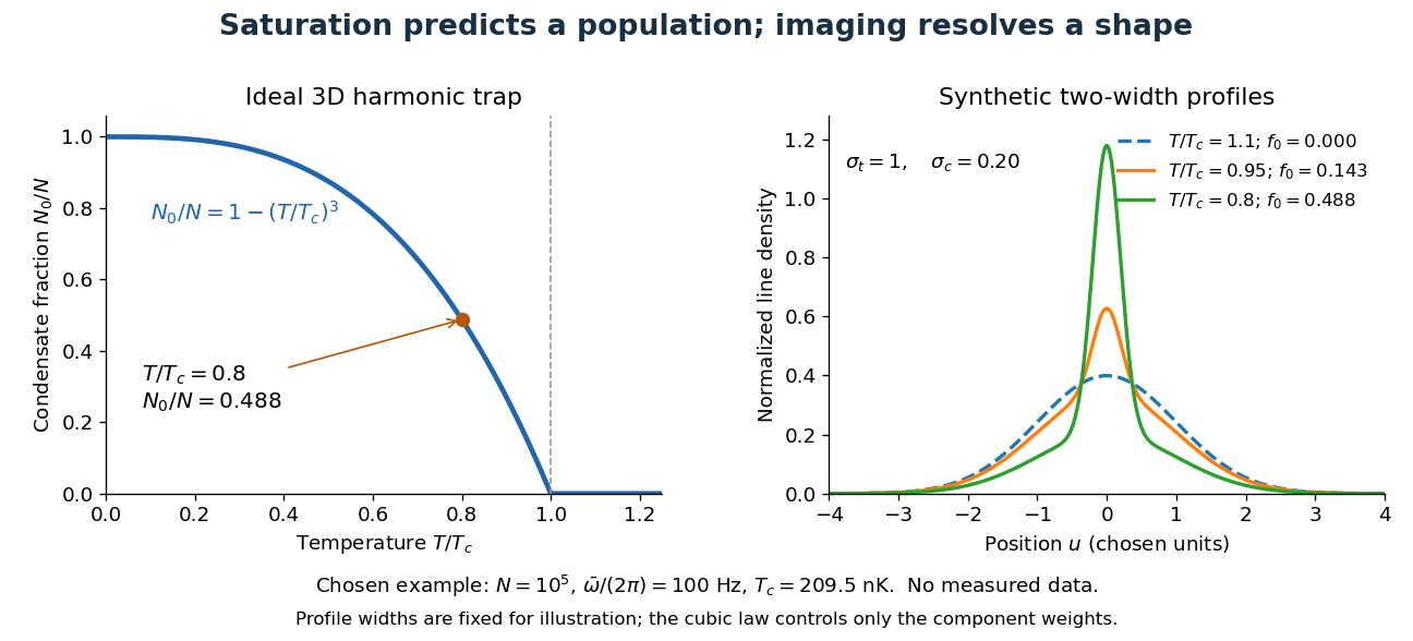

For absorption imaging in the weak-probe regime with negligible saturation, the optical depth is , where is the reference light intensity without atoms, the transmitted light intensity, an effective absorption cross section, and the column density. Integrating over both image coordinates gives the particle number; a central pixel height alone does not. Finite resolution can obscure a narrow component, and saturation invalidates this simple logarithmic calibration.
Bose condensation in a three-dimensional harmonic trap Created 2026-10-18 Updated 2026-10-20
Consider noninteracting bosons in one internal quantum state, at thermal equilibrium in the three-dimensional harmonic oscillator potentialHere is the mass, the positive are angular frequencies, and is their geometric mean. Measure the one-particle energy and chemical potential from the ground-state energy. The quantum harmonic oscillator levels then have with nonnegative integer and reduced Planck constant .
When , counting lattice points can be approximated by the volume of a tetrahedron in the positive octant of :This is a density of states, with units of inverse energy. The factor is the unit tetrahedron volume; differentiating produces the factor . Treat the single ground state separately: its macroscopic population would be lost by replacing every level with a smooth density of states.
For , integrate the Bose-Einstein distribution over excited energy eigenstates. As approaches zero from below, their maximum population isHere is the Boltzmann constant and the Riemann zeta function. A short proof uses and . The nonnegative terms permit exchanging summation and integration by Tonelli's theorem, giving . Near zero the integrand is proportional to , so its integral converges. That finite excited-state capacity is the mechanism of Bose-Einstein condensation.
Set . Particle conservation gives, to this continuum accuracy,Above , the macroscopic condensate fraction is zero and the chemical potential adjusts below zero. This cubic power belongs to a three-dimensional harmonic trap; it is not the homogeneous three-dimensional ideal gas exponent. For , and , the model gives . At , , or approximately condensed bosons. These are chosen parameters and calculated values.
Finite gives a smooth crossover rather than a sharp phase transition. The exact ideal gas sum over excited quantum harmonic oscillator levels differs from the continuum integral, especially when is not large relative to every . A sharp trapped-gas limit takes , with fixed and fixed frequency ratios. Interactions also alter the critical temperature, condensate fraction and release profile; a dilute gas can have appreciable interaction energy compared with the trap level spacing. The cubic law is a useful baseline, not a fit guaranteed for either 1995 experiment.
Thomas-Fermi screening 2026-10-18
In the long-wavelength static response of a degenerate conductor, a small electric potential changes the electron density by , where is the spin-summed density of states per volume per energy. The induced charge is therefore . With background permittivity , Poisson equation becomesA point charge then has . Larger electronic density of states gives stronger screening. This local response approximation does not capture the microscopic oscillatory tail of Friedel oscillations.[ref]
https://www.damtp.cam.ac.uk/user/tong/em/el6.pdf. Sections 7.7.3–7.7.5: Thomas-Fermi screening and its nonlocal corrections
Friedel oscillations Created 2026-10-18 Updated 2026-10-20
The sharp Fermi surface gives a nonlocal oscillatory electronic response around an impurity. In a three-dimensional isotropic metal its far-field oscillations have characteristic wavevector and algebraically decaying amplitude. They are absent from the purely exponential Thomas-Fermi screening potential. The local screening formula is a useful long-wavelength model, not an exact asymptotic expression at every distance.
Ruby pressure scale 2026-10-18
The ruby pressure scale converts a shift of a ruby fluorescence spectral line into pressure. Excitation light produces a fluorescence emission spectrum; fitting its line gives a wavelength . The reference must be measured or assigned at specified reference pressure and temperature. The difference is an observable; interpreting it as pressure requires a pressure calibration and suitable stress conditions.
The original 1972 report found sharp emission shifting toward lower photon energy as pressure increased; it tentatively associated broadening with nonhydrostatic conditions.[ref]
Pressure Measurement Made by the Utilization of Ruby Sharp-Line Luminescence by Richard A. Forman and others. Abstract: direction of R-line shifts and tentative nonhydrostatic interpretation
In use, excitation rejection, a calibrated wavelength axis and a fitted background matter because leakage or background can move an apparent peak. A brighter trace improves counting statistics but does not alone establish a correct pressure scale. Diamond anvil culet 2026-10-18
A diamond anvil culet is the small flat contact face at the tip of a diamond anvil. Its diameter determines its nominal surface area . The gasket hole has a different surface area ; neither should be confused with the much larger drive mechanism. For an ideal static axial balance, is the compressive force on either anvil. The two equal opposing loads do not produce through a single contact.
For an original chosen geometry, and giveHere is the mean axial contact stress over the culet, not a measured chamber pressure. Using a hole instead would give , nine times larger. That substitution falsely assigns the entire applied force to the hole.
To see the missing load path, idealize the culet as a coplanar hole region plus a surrounding contact annulus. With a hydrostatic chamber pressure and axial resultant carried by the gasket, its force balance isIf the stipulated chamber pressure is , the hole carries only and the gasket carries . These are model loads, not measurements. Real gasket deformation and anvil elasticity alter the local contact stress; the scalar balance cannot predict without additional information. This is why internal pressure calibration matters even when applied force is accurately known.
Debye wavevector Created 2026-10-18 Updated 2026-11-05
The spherical cutoff in the three-dimensional Debye model preserves three vibrational modes per atom. For atom density , and in a single-speed approximation. A monovalent free-electron metal has , giving . This cutoff is a mode-counting approximation, not an exact spherical boundary of the crystal's Brillouin zone.
Debye heat capacity 2026-10-18
The three-dimensional Debye model normalizes its phonon density of states to modes: below the Debye frequency . The thermal energy is . Differentiate at fixed volume and substitute to obtain the displayed heat capacity at constant volume.
At , integration by parts gives . Therefore . At , each mode approaches the equipartition theorem value of heat capacity, so , the Dulong-Petit law. Fixed harmonic zero-point energy does not contribute to either limit.
High-temperature phonon number in the Debye model Created 2026-10-18 Updated 2026-10-20
For three-dimensional Debye model mode density , the Bose-Einstein distribution becomes when . Integrating the occupations gives . The number of phonon quanta is not the number of vibrational modes and need not be bounded by it. If a stipulated electron-phonon scattering model makes resistivity proportional to this phonon number with a temperature-independent coefficient, the high-temperature electrical resistivity is proportional to .
Faithfulness criterion for a block representation of the cyclic group of order four Created 2026-10-18 Updated 2026-11-05
For real , this matrix defines a group representation of exactly when . Indeed its lower block satisfies , so exactly when . If , , so its order is four and the representation is faithful. If , its order is exactly two and the kernel of a group homomorphism is , giving an unfaithful representation. Other values do not give representations at all, including , when the proposed matrix is singular.
Two broad perfect conductors of width , separated by gap , carry opposite steady electric currents and connect through a terminating resistor . Away from edges, Ampère's circuital law and the superposition principle give gap magnetic field magnitude . Each conductor is an equipotential, and Ohm's law sets their electric potential difference to . Planar symmetry and charge-free Gauss's law then give uniform gap electric field magnitude . Injection parallel to the upper current makes the electric and magnetic Lorentz forces opposite. Their cancellation selects speed independent of nonzero electric charge and of operating current; nonrelativistic kinetic energy is .
Photoelectric contact-potential correction Created 2026-10-18 Updated 2026-10-20
Define as positive when the contact field adds to the retarding barrier, and let be the signed externally imposed retarding voltage. In this chosen sign convention the barrier is , henceThis convention specifies a model of the gap; an instrument's polarity labels must be translated into it. With a fixed , subtraction at two frequencies removes both the work function and the offset:For an original example with the same and an additional , choose and . The predicted terminal endpoints are and . The negative first endpoint calls for a small externally accelerating voltage because the contact field already over-retards the fastest electrons. Their difference is , giving . Ignoring in the intercept would falsely infer for the work function. The terminal line's zero would then be mistaken for a material threshold. If drifts between the two readings, even the slope is biased. These are calculated examples, not Millikan's measurements.
There are unlisted articles, also show them or only show them.