
Error bound for composite Simpson's rule 2026-10-18
Suppose has a fourth derivative that is a continuous function on the interval , and there. With , the signed quadrature error here is . Then, for some point ,In particular, a strictly positive fourth derivative makes : composite Simpson's rule overestimates the integral.[ref]
The bound's scale follows by adding the panel errors. A panel of width has signed quadrature error and absolute error at most . There are panels, so the triangle inequality gives . The intermediate value theorem for the continuous fourth derivative replaces the average of the panel values by a single value , giving the signed formula.
The underlying single-panel calculation can be seen through the Peano kernel theorem. On the interval , define the raw Peano kernel , where is integral minus Simpson's rule and is the positive part. Then for and for . It is strictly negative inside the interval and has integral . ThusThe uniform norm bounds the fourth derivative. The polynomial attains equality. Scaling to endpoint spacing multiplies the coefficient by , giving the sharp single-panel bound . The normalized Peano kernel is , so the external factorial must be omitted when using that normalization.
For the exponential function on , , so and the bound is . Its leading actual absolute error is , smaller than the bound because a uniform upper bound on the fourth derivative does not use its variation across the interval. The theorem bounds truncation error with exact function evaluations; sample errors and roundoff error are additional contributions, as described by noise sensitivity of a quadrature rule.
Primary beam Created 2026-10-18 Updated 2026-10-20
The primary beam is the individual antenna pair's directional sensitivity envelope in the complex visibility equation. For identical, identically pointed elements it is the individual element's power pattern. Its angular width sets the useful field of view; the much longer interferometric baselines set finer measured scales. The primary beam and the dirty beam describe different responses.
Positive difference of independent exponential waiting times Created 2026-10-18 Updated 2026-11-05
Let be independent random variables with exponential distributions of respective positive rates . Condition on and use the survival function of :At this is . Dividing by that probability proves that the positive difference conditional on again has an exponential distribution with rate . The memorylessness of the exponential distribution persists after an independent competing event has already occurred. Replacing the difference by a negative sentinel when adds an atom of a measure of mass at that sentinel without changing the positive tail.
Centralizer of a nonscalar two by two matrix 2026-10-18
For any real nonscalar matrix , its commuting matrices are exactly with . There is a vector for which form a basis: otherwise every nonzero vector would be an eigenvector, and applying this to two independent vectors and their sum would force to be scalar. Given a commuting , uniquely write . Then , so and agree on a basis and are equal. Conversely every polynomial in commutes with it. This generalizes the centralizer of a planar quarter-turn; the scalar-matrix exception is essential, because every matrix commutes with a scalar matrix.
Rotatory power 2026-10-18
The rotatory power is the rotation of transmitted linear polarization per unit path length, in . With equally transmitted circular eigenmodes and time convention , their accumulated phase difference gives . For uniform circular birefringence, . Generic linear birefringence need not admit one rotation angle common to all incident polarization directions. In a weak longitudinal Faraday effect, , with signed Verdet constant .
André-Louis Cholesky developed his calculation in the setting of geodetic adjustment: measured angles and lengths must satisfy geometric relations, while corrections should be small. The manuscript reproduced in Claude Brezinski's study is titled Sur la résolution numérique des systèmes d’équations linéaires and ends with the date 2 December 1910 at Vincennes. The manuscript reports a 56-equation calculation adjusting altitudes in an Algerian triangulation network. Its date establishes when this written account existed, rather than an exact invention date.[ref]
La méthode de Cholesky by Claude Brezinski. Claude Brezinski, La méthode de Cholesky, printed pp. 210–211: geodetic least-squares corrections; p. 217: manuscript title and caution about invention date; §4, p. 229: reproduced manuscript's 56-equation adjustment and closing date
A related algebraic reason for the method's usefulness is that normal equations involve a Gram matrix. If a real matrix has linearly independent columns, thenso is a positive-definite matrix. That gives the structure needed by a Cholesky decomposition. The historical adjustment problem instead produces from independent constraint rows; the same argument applies to its transpose. In numerical least squares, explicitly forming normal equations squares the condition number of a full-column-rank design matrix; a QR decomposition can therefore be preferable for accuracy. Indeed, the extreme singular values give . The factorization remains useful when a positive-definite matrix is already the natural input.
Cholesky decomposition as a sum of squares Created 2026-10-18 Updated 2026-10-31
For any real vector , a Cholesky decomposition gives the quadratic form identitySince is an invertible matrix, this squared Euclidean norm is positive whenever . The factorization thus certifies positive definiteness and gives coordinates in which the quadratic form is a sum of ordinary squares. For the matrix above,The level set is an ellipse; the linear map sends it to the unit circle. The points and go to and , respectively.
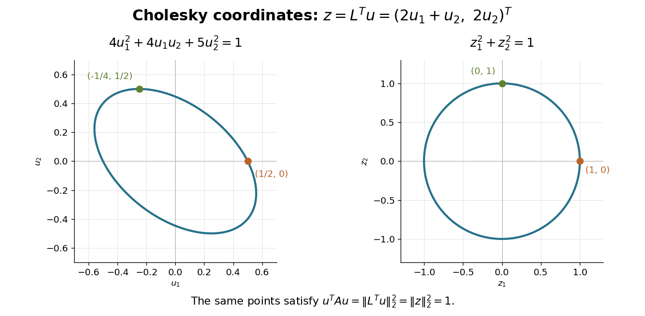

The same factor works in the reverse direction for Gaussian random vectors. If has independent unit-variance, zero-mean Gaussian random variables as coordinates, has covariance matrix . In this example and : their variances are and , while their covariance is . This is a concrete way to generate specified correlations from independent draws.
A triangular factor is not generally a square root of a matrix in the sense . Here . The Cholesky decomposition uses the product with the transpose, which is also what makes the quadratic form a squared Euclidean norm.
Electron mobility Created 2026-10-18 Updated 2026-10-20
The positive electron mobility relates the drift velocity of conduction electrons to an electric field: . In the isotropic Drude model, , where is the momentum relaxation time and the band effective mass. The minus sign describes negative charge; the electron mobility itself is positive.
Logarithmic change of variable in a Sturm-Liouville problem Created 2026-10-18 Updated 2026-10-31
For a Cauchy-Euler equation, logarithmic coordinates turn scale changes in into translations in . With , the chain rule gives and . Consequently the Sturm-Liouville operator becomes . Its natural weighted inner product has measure , so this change of variable also preserves the norm when the transformed problem uses ordinary integration in . On with Dirichlet boundary conditions, the orthonormal eigenfunctions are and the eigenvalues are , for .
Bragg crystal reflection experiment of 1913 2026-10-18
William Lawrence Bragg introduced the plane interpretation; his father William Henry Bragg built the X-ray spectrometer. Their joint 1913 paper, The Reflection of X-rays by Crystals, reports the experiment. [ref]
The Bragg law (University of Leeds Library Special Collections). The Bragg law: Lawrence's 1912 interpretation and the angle convention
[ref]William Bragg's spectrometer (Royal Institution collection). Description: William Henry Bragg designed and made the spectrometer
An X-ray tube supplied radiation through lead slits to a crystal mounted with its cleavage face through the rotation axis. A rotating ionization chamber replaced a spectrometer telescope; electric current measured the scattered signal, and a circular scale supplied angular readings. They first scanned the chamber at fixed crystal orientation, then swept crystal and chamber together to follow the reflection. [ref]
The Reflection of X-rays by Crystals by William Henry Bragg and William Lawrence Bragg. Bragg and Bragg (1913), pp. 428–430: preparation, source, slits, chamber, angular scale and scanning
Changing chamber gas checked detector dependence; readings on opposite sides checked face-setting errors. Repeated peaks with sines of half-deflections in integer ratios, together with matching absorption coefficients, distinguished repeated diffraction orders of the same wavelength from different radiation components. Comparing crystal faces constrained interplanar spacings. Their limits included slit broadening, face alignment and incomplete interception at glancing incidence; assigning absolute wavelengths still required a structural choice for . [ref]
The Reflection of X-rays by Crystals by William Henry Bragg and William Lawrence Bragg. pp. 428–430: gas and alignment controls; pp. 435–437 and Fig. 3: order comparison, absorption test, finite-face limitation and spacing ambiguity
Primitive cubic Bragg peak positions 2026-10-18
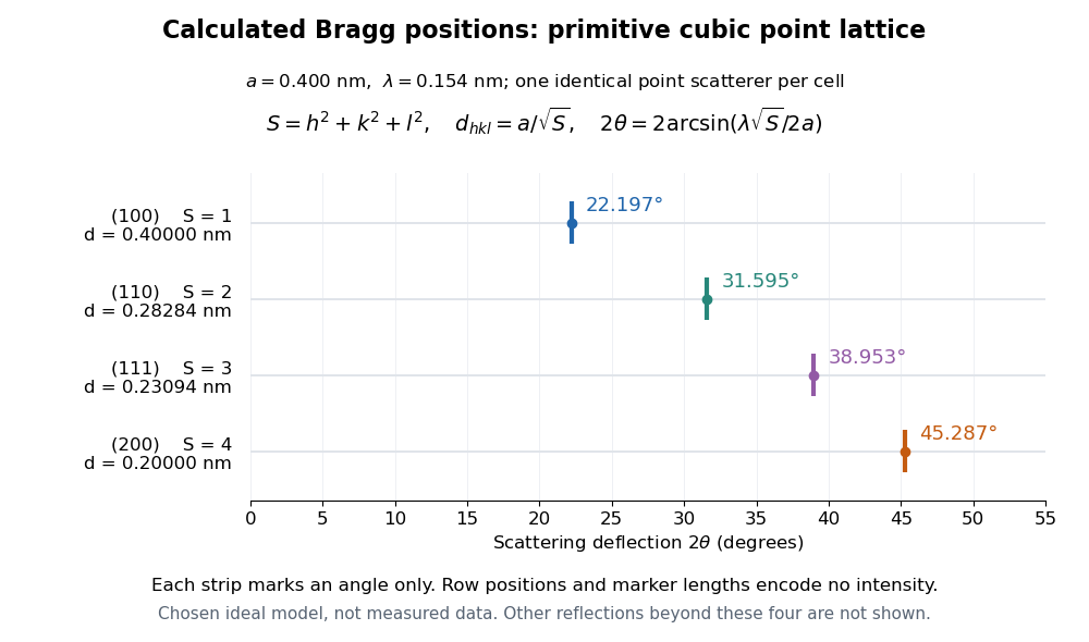
Consider a chosen primitive cubic lattice with and one identical point scatterer per primitive unit cell. Retain the incident wavelength . This is an ideal point model. Its reciprocal lattice vectors are for integer triples other than . Write . The associated interplanar spacing and first-order Bragg angle satisfyThe reflection labels use the Miller index convention, keeping unreduced triples to encode diffraction order. With that convention, set in Bragg's law for each label. The reflection is equivalently the second diffraction order of : does not imply extra scatterers halfway between the occupied planes. Counting both descriptions as distinct reflections would count the same direction twice.
For , , and , respectively, and the calculated interplanar spacings are , , and . Their calculated deflections are , , and . Equal steps in give equal steps in , not equal steps in . This regularity makes an angular pattern a test of a proposed crystal structure.

A real crystal structure has a Bravais lattice together with an atomic basis of a crystal. The crystal lattice structure factor selects the periodic directions; the crystal basis structure factor combines the scattering amplitudes of atoms within a unit cell and can cancel a reflection. Consequently Bragg's law alone predicts neither allowed reflections nor their wave intensities. [ref]
Structure factor. Online Dictionary of Crystallography by International Union of Crystallography; Definition, sum over atoms in the unit cell; Derivation, addition of companion atoms
Systematic absences further restrict observed families; for example, face-centered cubic lattice centering permits only indices all even or all odd in conventional cubic indexing. The four strips above apply to the stated primitive cubic lattice, not to sodium chloride or a face-centered cubic lattice. [ref]Reflection conditions. Online Dictionary of Crystallography by International Union of Crystallography; Definition and Table 1: primitive versus all-face-centered integral reflection conditions
Bragg path difference 2026-10-18
Compare two rays scattered into parallel outgoing directions from neighboring lattice planes. In the diagram, lies on the upper plane and on the lower plane, directly beneath with . Draw through the incoming and outgoing equal-wave phase fronts, perpendicular to their respective rays. They meet the lower ray at and . Each right triangle gives , so the lower ray travels the extra distanceThe resulting phase difference is . Constructive interference requires , which proves Bragg's law in this ray construction. Comparing equal-wave phase fronts, rather than arbitrary ray endpoints, is what makes the distance comparison meaningful.
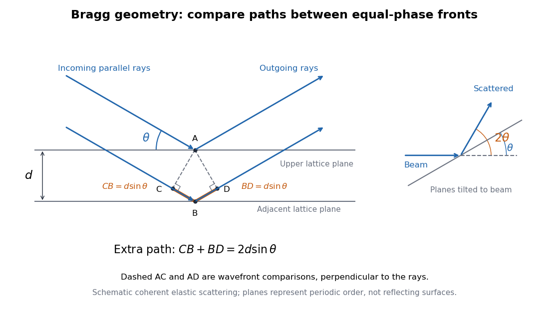
Bragg rays, extra path, and the distinction between the glancing angle and scattering deflection
. Original schematic of coherent elastic scattering. The orange segments give the extra path ; dashed segments compare equal-wave phase fronts. The separate angle sketch shows why the outgoing beam is deflected by when the Bragg angle is . The illustrated angle is schematic. Details.
The same geometry connects to the reciprocal lattice. With wavenumber , the elastic Bragg scattering condition gives a transfer magnitude . A reciprocal vector normal to these lattice planes has . Equating them again yields Bragg's law. The ray and reciprocal lattice descriptions therefore express the same wave phase matching.
Bragg angle 2026-10-18
The Bragg angle is the glancing angle from the incident beam to the selected lattice planes, with . If is instead the angle from the beam to the plane normal, and Bragg's law becomes . Defining the angle explicitly prevents a sine-versus-cosine error as well as a factor-of-two error in the detector deflection.
Choose and as an illustrative model, not historical measurements. For the first diffraction order,The second diffraction order has and ; the third would require and is impossible. These are different diffraction orders of the same interplanar spacing at the same wavelength.
Conversely, a first-order reflection at a measured deflection gives the interplanar spacingUsing recovers . This is the useful reversal: a known wavelength turns an angular measurement into an atomic length. An unassigned diffraction order or an unknown wavelength prevents that single measurement from determining uniquely.
2-satisfiability 2026-10-18
2-satisfiability restricts SAT to CNF in which each Boolean clause has at most two Boolean literals. The example in Boolean satisfiability problem is therefore a 2-SAT instance. Unlike general SAT and 3-SAT, 2-SAT has a polynomial-time algorithm; its tractability concerns finding a satisfying assignment or deciding that none exists, not merely checking a candidate. 3-SAT allows up to three Boolean literals per Boolean clause and is NP-complete, even though it includes many individually easy instances such as this one.[ref]
The key logical equivalence iswhere are Boolean literals. It expresses a two-Boolean literal Boolean clause as two logical implications. Representing these logical implications as edges in a directed graph gives a route to the polynomial-time algorithm. In the example, says both and : enabling the feature requires its component, and an absent component excludes the feature.
Partial Boolean assignment 2026-10-18
A partial Boolean assignment gives truth values to some of a Boolean formula's Boolean variables. An extension is a complete Boolean valuation agreeing on the assigned Boolean variables. In CNF, a Boolean clause containing a true assigned Boolean literal is already satisfied; a Boolean clause whose every Boolean literal is assigned false rules out all extensions. A Boolean clause with no true assigned Boolean literal and at least one unassigned Boolean variable is unresolved. An unresolved Boolean clause need not have a compatible extension with the other Boolean clauses.
For in Boolean satisfiability problem, setting already falsifies , so both choices of can be discarded. Setting only leaves unresolved and forces if a satisfying assignment is to survive; then forces . Branching on an unassigned Boolean variable into its two truth values and discarding branches with a false Boolean clause is sound: every satisfying assignment follows one branch and cannot extend a false Boolean clause. If all branches are eliminated, the original Boolean formula is an unsatisfiable Boolean formula.
Unsatisfiable Boolean formula 2026-10-18
An unsatisfiable Boolean formula has no satisfying assignment. Forthe Boolean valuation falsifies the first Boolean clause, and falsifies the second. Both possible truth values fail, proving
UNSAT. Each Boolean clause alone has a satisfying assignment, but their logical conjunction does not: compatibility is the central issue. By contrast, finding just one failed Boolean valuation for a general Boolean formula only rejects that candidate. Finding one successful Boolean valuation proves SAT; proving UNSAT requires excluding every candidate, possibly with a compact argument rather than a full truth table. Satisfying assignment Created 2026-10-18 Updated 2026-10-25
A satisfying assignment is a complete Boolean valuation for which a Boolean formula has truth value one, written . The notation describes a relation between the Boolean valuation and the Boolean formula. For the example in Boolean satisfiability problem, is a model of a Boolean formula , whereas is not. SAT asks for existence of at least one satisfying assignment, rather than for every Boolean valuation to work; the latter condition makes a tautology.
Boltzmann encoder demonstration 2026-10-18
David H. Ackley, Geoffrey Hinton and Terrence J. Sejnowski tested their 1985 algorithm on a simulated 4–2–4 encoder. Two four-unit visible groups communicated through two hidden units, with no direct connections between the groups. Preparation set weights to zero and supplied corresponding one-active-unit patterns. Noisy clamping and annealed settling generated pair-coactivation readouts, compared with freely running readouts to choose weight changes. Learned hidden codes were the outcome. Equal sampling effort in clamped and free conditions supplied the comparison; noise limited weight growth. Finite settling was assumed to reach equilibrium, limiting the evidence for exact likelihood learning.[ref]
Two-spin Boltzmann learning 2026-10-18
Take two visible bipolar units, no hidden units, zero thresholds, , and . As original training data, assign probabilities each to and and each to and . The data pair product averages to . Enumeration of all four states gives two weights and two , hence the partition function andStarting at , the positive-minus-negative difference is . A gradient ascent step of size gives . Each aligned state now has probability and each opposed state , bringing the model toward the data. The log-likelihood increases from to . Solving gives , which reproduces the data exactly. Since , this is the unique maximum. These are exact enumerations and their decimal evaluations, with no sampling or laboratory measurements.
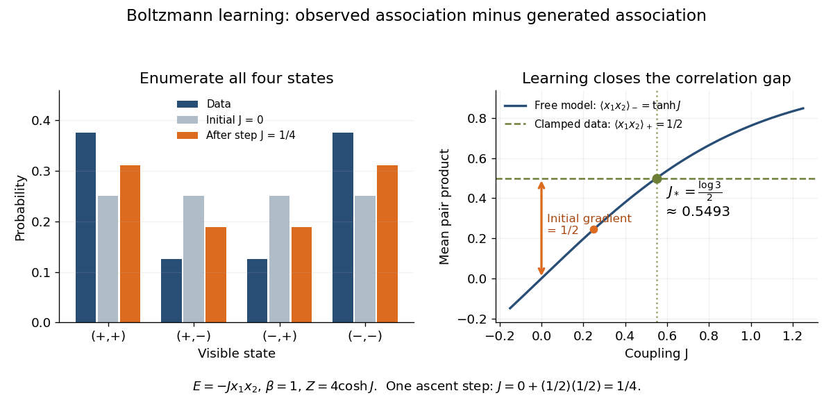
Exact probabilities and positive-minus-negative learning for two visible units
. Left: data and model probabilities before and after one gradient ascent step. Right: the data pair-product average and the model average determine the log-likelihood derivative; their intersection gives the optimal coupling. Details.
Split the units into visible units , whose patterns occur in the training data, and hidden units . Let be the empirical probability distribution and maximize the average log-likelihood , where . The positive phase clamps to data and averages over ; the negative phase releases all units and averages over . The displayed difference uses these two expectations. When both units are visible, the positive pair product is supplied directly by the data.
For a proof, write . Differentiating each finite sum gives, respectively, and . Since , subtraction proves the rule. Similarly . A small positive step along these gradients increases log-likelihood. The negative term suppresses associations overproduced by the model; strengthening observed pairs alone misses this correction. The identity requires equilibrium expectations; estimates from insufficiently mixed sampling can give a biased update.
There are unlisted articles, also show them or only show them.