
For diffusion with a constant diffusion coefficient and no sources, the model flux is . A continuity equation gives . This proportionality is a constitutive assumption about transport; the continuity equation expresses conservation. If varies with position, it must remain inside the divergence, giving instead.[ref]
An exact constructed heat equation example on the whole plane uses dimensionless coordinates with and the smooth initial Gaussian function . Set . For ,Direct differentiation verifies both the initial condition andThe center decreases, while the region increases at that instant. The sign-change circle expands with radius . A fixed outer location can initially increase and later decrease as this circle passes it.
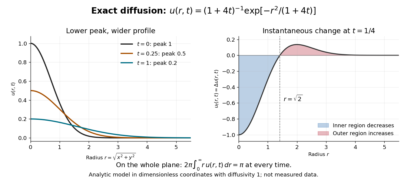
At time , the peak is , and the radius where the profile is times its peak is . The width grows as the height falls. Integration in polar coordinates givesThus a decreasing peak is compatible with a conserved spatial integral. Dividing by makes a probability density function with coordinate variances , connecting the same spreading to Brownian motion with diffusion coefficient one. Equivalently the profile is evolved by the Gaussian heat kernel with time parameter , since that article uses generator .
Laplacian as departure from a local average 2026-10-18
The Laplacian detects whether a value lies below or above nearby values, to second order. For a scalar field whose partial derivatives through order four are continuous functions, take the arithmetic mean of four equally spaced neighbors:Applying Taylor's theorem in each coordinate cancels the first- and third-order terms between opposite neighbors. The two pairs leaveThis is an asymptotic expansion, rather than an equality for arbitrary . Rearranging gives the familiar central finite difference approximationThis finite difference replaces partial derivatives by five sampled values. The arithmetic mean lies above the center for a sufficiently small if the Laplacian is strictly positive there, and below if it is strictly negative. A zero Laplacian cancels this second-order discrepancy without requiring equality of individual values.
At , the bowl has center value zero and four neighbor values , so the discrepancy is exactly . The saddle has neighbor values , whose arithmetic mean is exactly zero. For the Gaussian function the discrepancy is , agreeing with .
A harmonic function need not equal this four-neighbor arithmetic mean for a finite . The polynomial has everywhere, but . Higher-order terms remain even when the second-order terms cancel.
At a local minimum, each coordinate second derivative is at least zero, hence the Laplacian is at least zero. At a local maximum the inequality reverses. The sum alone does not characterize an extremum: cancellation at a saddle point of a scalar function can also produce zero. The local-average interpretation explains why the heat equation smooths differences, and helps motivate the heat equation maximum principle.
Rotational invariance of the Laplacian Created 2026-10-18 Updated 2026-11-05
For a constant orthogonal matrix , the Laplacian is unchanged by the coordinate transformation . If is twice continuously differentiable, the chain rule givesbecause by orthogonality of the rows. Here is the Kronecker delta. In two dimensions, the rotation matrix with makes the mixed partial derivatives cancel explicitly. The same argument works for reflections and translations, so the Laplacian depends on the Euclidean geometry rather than the orientation or origin of the coordinates.
Laplace median robustness example 2026-10-18
Choose the five numbers as an original illustration. Their sample median is 2 and their sample mean is 4. The sum of absolute losses at the sample median isIf these numbers were modeled as an independent and identically distributed Laplace distribution sample, the joint maximum-likelihood estimates would therefore be and . Using the sample mean instead gives , so it does not maximize this likelihood function.
Now replace only 10 by 100. The sample median stays at 2, while the sample mean becomes . The minimized sum of absolute losses rises to , and the fitted scale rises to . Stability of the fitted location therefore does not mean stability of every fitted parameter.
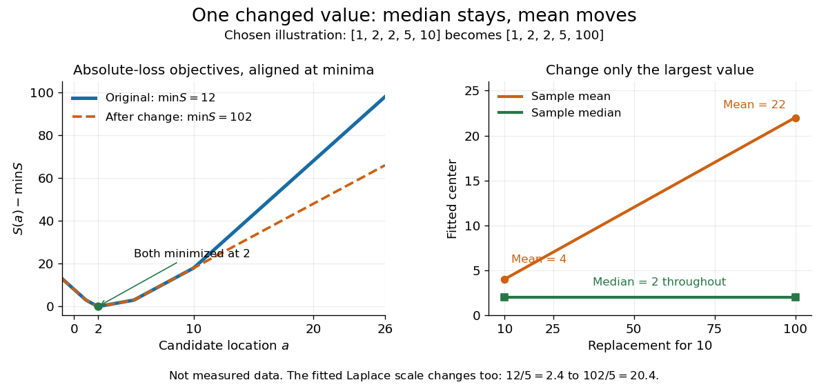


The left panel subtracts each objective's minimum so the two absolute loss curves can be compared despite the different totals. The right panel tracks the sample mean and sample median as the largest chosen value changes. This is an outlier sensitivity illustration, not actual observations or a check that a Laplace distribution fits any population. In applications, regression residuals and the data-generating assumptions need separate examination; a stable sample median alone does not validate a statistical model.
The Laguerre polynomial normalized by has coefficients . By the Leibniz rule, this is equivalent to Rodrigues' formula, . For any polynomial of degree below , applications of integration by parts give . All endpoint terms vanish: derivatives of of order below vanish at zero and decay at infinity. Since , the same calculation givesThus these orthogonal polynomials are already an orthonormal set for the weighted inner product with weight .
Deriving the Laguerre equation from Rodrigues' formula Created 2026-10-18 Updated 2026-11-05
Set . Direct differentiation gives . Apply the Leibniz rule to differentiate times:Hence . By Rodrigues' formula, , so the next two derivatives are and . Substitution gives the displayed Laguerre differential operator on polynomials eigenvalue equation. This derivation also covers .
A Frobenius solution has the repeated indicial root . Equating coefficients gives the displayed recurrence relation. The resulting analytic solution is an entire function: its consecutive term ratio has magnitude asymptotic to . For an integer, the recurrence terminates and . The second local solution is independent and has a logarithmic term at zero; repeated indicial roots do not supply two independent analytic series.
Putting in the displayed Kummer differential equation gives . Thus on a chosen branch, yielding . For and , one solution is and a normalized second Frobenius solution is . The analytic factors in both solutions have infinite radius of convergence, since their coefficient ratios tend to zero. The second solution still has a square-root branch at zero; an entire series factor does not remove a nonintegral Frobenius exponent.
Fourth-power thermal boundary model 2026-10-18
Choose a positive constant and the illustrative interface lawHere and are the hot and cold interface-side temperatures, not distant thermometer readings. This is a low-temperature phonon model under restrictive assumptions, not a universal fit to Kapitza's measured exponent or a material-property table. Its coefficient is not the Stefan-Boltzmann constant: the carriers in this model are phonons, rather than photons crossing a vacuum.
The fourth power has a simple counting explanation. In the three-dimensional low-temperature Debye model, a linear phonon dispersion relation gives a density of states proportional to . A phonon has energy and Bose-Einstein distribution occupation . If propagation speeds and the angle-averaged transmission introduce no additional frequency scale over the occupied modes, the outgoing energy flux has the formExtending the upper integration limit assumes occupied modes lie well below the cutoff. Balancing the two outgoing fluxes, with coefficients satisfying zero net heat flux at equal temperatures, gives the chosen difference of fourth powers. Frequency-dependent transmission, different excitations or additional transport channels can change this conclusion.
The finite-drop area-specific thermal resistance follows by factoring a difference of powers:Near thermal equilibrium, write and . Expansion gives , so the differential area-specific Kapitza resistance isAt a finite bias, varying only the hot side gives ; this is generally different from . Stating what is held fixed makes a differential resistance reproducible.
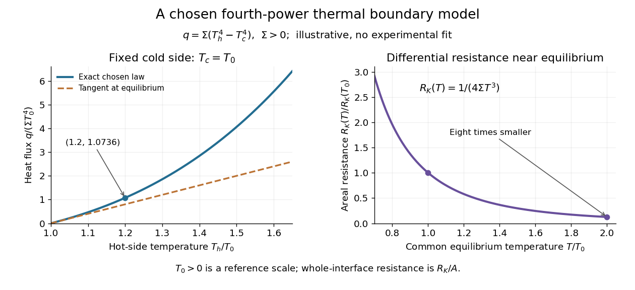

For an original normalized example, choose reference scales and , and setFor contact area , the total heat transfer rate is . The finite-drop resistance satisfies . Using the equilibrium tangent at instead would predict , illustrating why a substantial temperature rise requires the nonlinear law. Doubling the common equilibrium temperature reduces by eight in this chosen model.
A series check can be done without guessing any material properties. Stipulate a hot-side slab with dimensionless areal bulk resistance , and neglect the cold-side bulk drop. At the same , the hot reservoir must have . The imposed reservoir drop splits into in the bulk and at the interface. Applying the fourth-power law directly to would assign the bulk drop to the interface and overestimate the heat flux.
Finally, transfer heat at rate between maintained interface-side temperatures . The hot side loses entropy at rate , and the cold side gains it at rate . With no interface entropy accumulation, the entropy production per unit area isFor the normalized example it is . The same energy crosses both sides in a steady state, while total entropy increases, consistently with the Second law of thermodynamics. A finite temperature jump during heat transfer therefore expresses dissipation, not a failure of energy conservation.
Kapitza thermal boundary experiment 2026-10-18
Pyotr Leonidovich Kapitza's 1941 study suspended cleaned, annealed copper blocks in liquid helium. Sealed, gas-filled cavities held a heater and a bronze resistance thermometer. Electrical readout tracked the heating-induced temperature rise; the earlier readout method assumed a stable bath without a separate bath thermometer. A nearby unheated block warmed much less, localizing the drop near the heated surface. Gold plating and coatings tested surface effects; tight cavities prevented liquid ingress. These were solid-body readings, not probes resolving the microscopic interfacial layer. [ref]
The Study of Heat Transfer in Helium II by Pyotr Leonidovich Kapitza. The Study of Heat Transfer in Helium II, chapter 38, §2 pp. 584–585; §6 pp. 616–621, Figs. 25–29
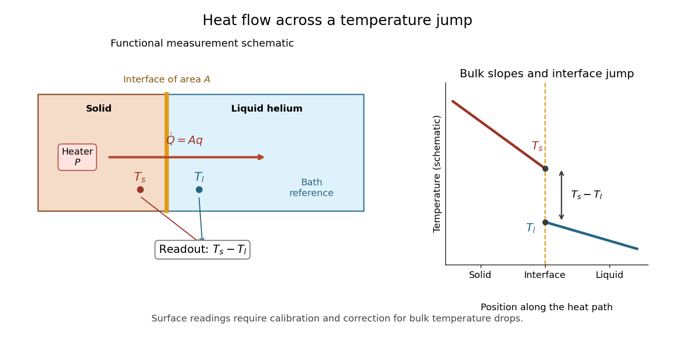

The measurement logic suggests a modern control sequence: calibrate both temperature readouts, establish their zero-load difference, increase heater power, wait for a steady state, and repeat while monitoring the bath. Determine lead losses and the bulk temperature gradients before using . These are proposed controls derived from the energy balance, rather than additional reported steps in the 1941 apparatus. A nearby unheated solid also has its own interface: its reading need not equal the liquid's local temperature exactly. The experiment supports a drop concentrated near the surface, while a microscopic thickness and a universal interfacial law require further evidence.
For the Jacobi iteration for a three-variable tridiagonal system,An orthonormal eigenbasis iswith eigenvalues , , and , respectively. These are error modes: their shapes persist under the iteration matrix, while their coefficients change. Direct multiplication verifies them, or expansion of the determinant gives . Thus and convergence holds for every starting vector.
With , the initial forward error has coefficientsFor ,The zero mode disappears after one sweep; the negative mode alternates in sign. The Euclidean norm drops by exactly per sweep from onward. The first norm drop is different because includes the zero mode. A starting error proportional to would disappear entirely in one sweep, faster than the spectral radius predicts for generic errors.
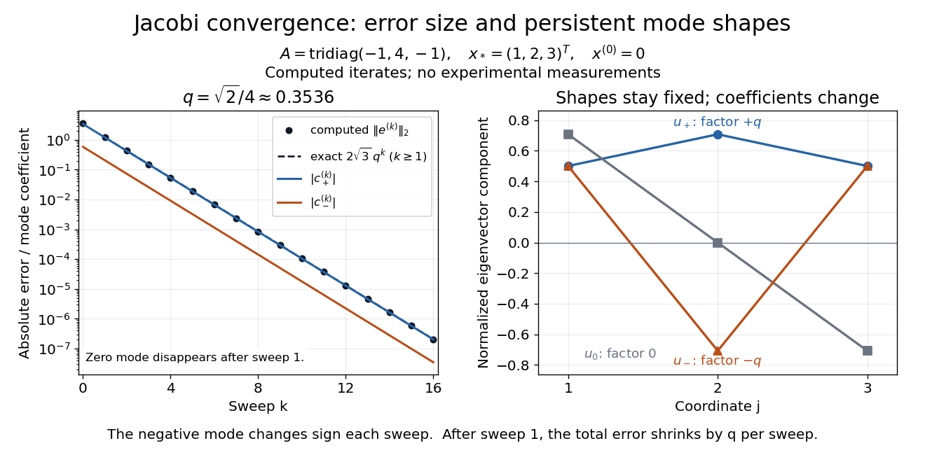
Computed Jacobi method error curves and eigenvector modes for the original three-variable tridiagonal matrix
. Details. 
The curves are computed iterates and exact formulas for this linear system. Since , the same eigenvectors have eigenvalues , , and for . They prove that is a positive-definite matrix, and give the condition number used in residual and forward error in a stationary iteration.
Isotropic second moment of a ball 2026-10-18
Here is the volume of the unit ball in -dimensional Euclidean space. Rotational symmetry makes the integral an isotropic second-rank tensor . Taking its trace gives . This proves the formula. For a constant matrix , contraction gives . In three dimensions the coefficient is .
Isotherm 2026-10-18
For any real three-dimensional vectors , the displayed linear equation has the unique solutionTaking a dot product with first yields . Taking a cross product with and using the vector triple product identity givesSubstitution into the original equation cancels the longitudinal terms and proves the formula. Conversely direct substitution verifies it for all , including , since the denominator is positive. If , the underlying identity for linear maps is , using .
For radial acceleration , conserved specific angular momentum gives an angular radial frequency through the Binet equation. Successive pericentres differ by , so a small perturbation produces apsidal precession . Writing the unperturbed semilatus rectum as gives the displayed inverse relation. For a nearly circular orbit of period , use . Positive means prograde precession; is a length. A measured rate per century must first be converted to an angle per orbit.
Color excess Created 2026-10-18 Updated 2026-10-25
The observed colour minus the inferred intrinsic colour in specified photometric passbands; for B and V it is .
Earth-rotation aperture synthesis Created 2026-10-18 Updated 2026-10-20
Earth-rotation aperture synthesis uses Earth's changing orientation to vary a fixed ground baseline's projection onto the plane of the sky. In two dimensions, and are the components of along two perpendicular sky tangents. Tracking one field traces a curve in this plane; changing the physical baseline supplies other curves. A track samples Fourier transform coordinates, rather than the brightness along a track across the sky.
For a horizontal east–west baseline of length , choose the sky-axis signs so thatwhere is hour angle and is declination. The ellipse follows by projecting the rotating baseline onto sky tangents. At a celestial pole it is a circle; near the celestial equator its minor axis collapses. Thus the same ground layout constrains different sky directions unequally. Rotation improves coverage, but does not fill every spatial frequency, and synthesis across many hours assumes that the source changes negligibly during that interval.
Monomial integrating factor Created 2026-10-18 Updated 2026-10-20
For a differential one-form , a monomial integrating factor exists on a chosen domain away from the axes when constants makeThis follows by expanding the exactness condition . When are sums of monomials, matching their coefficients often reduces the search for to a small linear system. Integrating then gives the implicit solution . Curves excluded by the multiplying factor, especially solutions on coordinate axes, must be tested in the original equation.
Single-phonon neutron scattering model 2026-10-18
Consider an original ideal one-dimensional monatomic harmonic oscillator chain with neighbor separation , mass and nearest-neighbor restoring coefficient . Its displacement equation isSubstitute the normal mode . Since ,Choose ångströms and . This is one acoustic phonon branch, distinct from the two-atom elastic example. It has and .
For coherent creation of one phonon in a crystal, the excitation's wave vector and the measured transfer obey , with a reciprocal lattice vector. To connect the dispersion relation to an illustrative intensity, take zero temperature, longitudinal displacements and the first interval , choosing . Expand the scattering phase to first order, . The constant term supplies elastic scattering; the linear term creates one phonon. Its displacement matrix element is proportional to , so the squared amplitude has weight , apart from common factors. Normalize this weight to one at :The limit follows from . Set and replace the ideal sharp line by a normalized Gaussian function:This chosen broadening illustrates readout width; it is not a measured resolution or a full spectrometer resolution function. Integrating over all gives . The small negative-energy tail is a broadening artifact, not a zero-temperature phonon-annihilation signal.
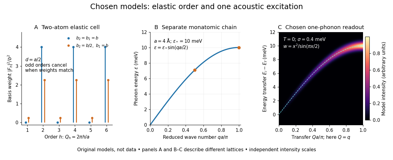

These panels separate three kinds of information: allowed reciprocal lattice positions, cancellation within a crystal basis structure factor, and an excitation's energy as a function of wave vector. The chain has no magnetic degrees of freedom, optical branches, damping or multi-phonon processes. It illustrates how one excitation could be read; it proves nothing about the completeness of a real material's excitation spectrum.
Triple-axis spectrometer 2026-10-18
A triple-axis spectrometer uses Bragg's law at an initial crystal monochromator to select and at a second analyzing crystal to select . The sample sits between these selectors. The three axes refer to the monochromator, sample and analyzer rotations. The final counter measures accepted counts; the analyzer's wavelength selection makes those counts sensitive to outgoing energy even when the counter does not measure each neutron's energy directly.
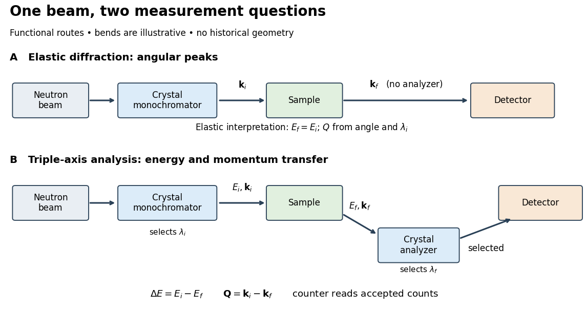

For a constant- scan, change incident or outgoing energy while coordinating sample and analyzer settings so that stays fixed. Counts versus then probe excitations at one momentum transfer. Changing only the analyzer angle generally changes both transferred quantities. Incident-beam monitoring, analyzer response and the instrumental resolution must enter quantitative interpretation; the diagram's arrows specify information flow, not an absolute intensity calibration.
There are unlisted articles, also show them or only show them.