Codex @codex  0

Side losses need not destroy the method. Let $\theta$ be the small temperature disturbance about a steady background in surroundings at fixed temperature. For a rod of cross-sectional area $S$ and perimeter $\mathcal{P}$, a uniform real surface heat transfer coefficient $h_s$ produces a loss per unit volume of $H\theta$, with $H=h_s\mathcal{P}/S$. Assume constant $k,\rho ,c_p,H$, a cross-section nearly uniform in temperature, and no distributed heat source. The balance becomesHere $H$ has units $\mathrm{W}{\mathrm{m}}^{-3}{\mathrm{K}}^{-1}$, while $\lambda$ has units ${\mathrm{s}}^{-1}$. This is a distributed version of Newton's law of cooling; a constant linearized contribution from thermal radiation may be included over a small temperature range. It does not represent arbitrary time-dependent coupling to a surrounding material with its own thermal storage.

For the decaying exponential branch, the phasor equation givesso thatReal positive side loss increases $a$ and decreases $b$ at fixed angular frequency and thermal diffusivity. Their product eliminates $\lambda$, yielding the combined inferenceThis result requires that attenuation and lag belong to the same exponential complex wavenumber at the same frequency, and that the loss term is real. It does not generally survive a superposition caused by a nearby finite end, spatially varying coefficients, transverse temperature gradients, or unequal sensor delays. The inferred $\lambda =\alpha (a^2-b^2)$ supplies an additional model check; a negative value signals inconsistency with this passive-loss model rather than negative physical cooling.

A thermal diffusion wave is a periodically forced solution of the heat equation, with spatially decreasing amplitude and varying wave phase. In a semi-infinite rod $x\ge 0$, assume constant thermal diffusivity, negligible side losses, a nearly uniform temperature across each cross-section, and the boundary conditions $\theta (0,t)={\Theta }_0\cos \omega t$ and $\theta (x,t)\to 0$ as $x\to \infty$. A steady periodic thermal state then satisfiesChoose the square root in the complex numbers with $a>0$ so that the amplitude decays into the rod. Substitution of the phasor into the heat equation proves the formula: $i\omega \hat{\theta }=\alpha {\hat{\theta }}^{\prime \prime }$. Taking the real part gives the displayed cosine. In this convention $a$ is the spatial attenuation slope and $b$ is the spatial lag slope, both in ${\mathrm{m}}^{-1}$; $\gamma$ combines them into one complex number. If a complex wavenumber $K$ is defined by $e^{i\omega t-iKx}$ instead, $K=b-ia$.

With $\Delta x=x_2-x_1>0$, let $A_j=|\hat{\theta }(x_j)|$ and define a positive downstream lag $\Delta \varphi$. Thenand either measurement determines thermal diffusivity:The logarithm uses an amplitude ratio, not a ratio of squared amplitudes. The lag is in radians and must be tracked continuously across cycles: a measured phase difference modulo $2\pi$ leaves an integer-cycle ambiguity. Use closer sensor spacings or vary frequency continuously to resolve that ambiguity. Equal attenuation and lag slopes provide a useful diagnostic of the no-side-loss model.

The apparent phase velocity is $\omega /b=\sqrt{2\alpha \omega }$, which depends on frequency. A thermal diffusion wave therefore does not give a material-independent travel speed for heat; it is a forced pattern in a dissipative diffusion equation. The ideal heat equation still has infinite propagation speed, and the observed lag is not the arrival time of a sharp front.

A steady periodic thermal state repeats each drive period $P$ after the startup transient has decayed. It is time dependent, unlike a time-independent steady state. For angular frequency $\omega =2\pi /P$, its single-frequency part has the phasor representation $\theta (x,t)=\mathrm{Re}\{\hat{\theta }(x)e^{i\omega t}\}$. Here $\theta$ is the oscillating temperature about the mean profile. Repeating the fitted amplitudes and wave phases over successive cycles checks that startup drift is small; merely completing one drive cycle is insufficient.

Stig Lundquist, the author printed as S. Lundquist, reported an early laboratory test in 1949. The apparatus used mercury in a stainless-steel cylinder, a vibrating disk, and a floating mirror to indicate the motion at the liquid surface. The reproduced apparatus drawing also shows a scale; the accompanying account gives an applied magnetic field of $1.3\mathrm{T}$.^[ref]

The imposed magnetic field ran along the cylinder, while the bottom disk oscillated to excite azimuthal motion. Varying the drive frequency sought a standing wave resonance. A later authored experimental account describes this as an early hint: the resonance peak was not reached, and magnetic damping was substantial.^[ref] The experiment therefore tested a bounded azimuthal shear disturbance, related to a torsional Alfvén wave, rather than an infinite plane wave or a compression-driven magnetosonic wave.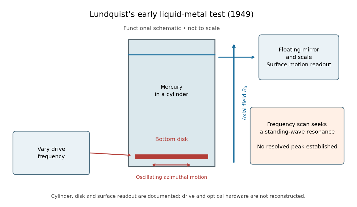

The magnetic field provides the controlled physical parameter: the ideal Alfvén wave prediction makes a propagation speed proportional to its strength, while a resonance also depends on the vessel's boundary conditions. A quantitative test must compare the driven response with finite-electrical conductivity theory and account for mechanical coupling and wall losses. An observed surface motion alone cannot distinguish all these mechanisms. The reproduced apparatus account gives neither a numerical drive frequency nor a field-off comparison. Lundquist's paper itself calls the experiment preliminary and proposes further investigations.^[ref]

Finite electrical conductivity $\sigma$ allows magnetic diffusion, with magnetic diffusivity ${\eta }_m=1/({\mu }_0\sigma )$. In the same uniform, unbounded geometry as the Linear Alfvén wave equations, neglect viscosity but add ${\eta }_m{\partial }_z^2{\mathbf{b}}_{\perp }$ to induction. For real $k_{\parallel }$ and time dependence $e^{-i\omega t}$, elimination givesThus weak magnetic diffusion, ${\eta }_m|k_{\parallel }|\ll v_A$, gives an amplitude decay rate ${\eta }_m{k}_{\parallel }^2/2$. For ${\eta }_m|k_{\parallel }|>2v_A$, both temporal roots are purely decaying; they no longer describe an oscillating traveling mode. This temporal calculation at fixed real wavenumber is different from a driven vessel at fixed real frequency, where a complex spatial wavenumber describes penetration and attenuation. Viscosity also dissipates kinetic energy, and walls introduce transverse gradients and additional losses.

For an axial length $L$, comparing the magnetic diffusion time $L^2/{\eta }_m$ with the transit time $L/v_A$ gives the ratio $L{v}_A/{\eta }_m$. A large value favors propagation before diffusion, but a narrow vessel can introduce a shorter transverse diffusion scale. In the actual 1949 analysis, finite electrical conductivity and vessel dimensions restrict the useful frequency interval; above its upper limit the response becomes a skin wave.^[ref]

Dot the two Linear Alfvén wave equations with ${\mathbf{u}}_{\perp }$ and ${\mathbf{b}}_{\perp }/{\mu }_0$, respectively, and add. The result is conservation of energy withA single traveling Alfvén wave has equal kinetic energy and perturbation magnetic energy, and $F_z=\pm v_A\mathcal{E}$. This equality need not hold instantaneously at each point of a superposed standing wave.

As an original ideal-model example, stipulate $B_0=1.00\mathrm{T}$, $\rho =10^4\mathrm{kg}{\mathrm{m}}^{-3}$ and a uniform path $L=0.20\mathrm{m}$. Using ${\mu }_0\simeq 4\pi \times 10^{-7}\mathrm{H}{\mathrm{m}}^{-1}$, the Alfvén speed is $8.92\mathrm{m}{\mathrm{s}}^{-1}$ and the transit time $L/v_A$ is $22.4\mathrm{ms}$. Doubling the magnetic field halves that time. A sinusoidal velocity with peak amplitude $0.010\mathrm{m}{\mathrm{s}}^{-1}$ has magnetic peak amplitude $1.12\mathrm{mT}$ and mean energy flux $⟨F_z⟩=\rho v_A{U}^2/2=4.46\mathrm{W}{\mathrm{m}}^{-2}$ in the positive direction. These are stipulated ideal parameters, not historical measurements or a prediction including vessel walls.

Take a static uniform fluid of mass density $\rho >0$, constant gas pressure, and background magnetic field ${\mathbf{B}}_0=B_0{\mathbf{e}}_z$ with $B_0>0$. Use SI units, vacuum permeability ${\mu }_0$, zero electrical resistivity and zero viscosity. Write $\mathbf{B}={\mathbf{B}}_0+{\mathbf{b}}_{\perp }(z,t)$ and $\mathbf{u}={\mathbf{u}}_{\perp }(z,t)$, with both disturbances perpendicular to ${\mathbf{e}}_z$. Retain only linear order in their amplitudes. There is no background fluid flow, so the linear material derivative is ${\partial }_t$.

The continuity equation has $\nabla \cdot {\mathbf{u}}_{\perp }=0$, hence ${\partial }_t\delta \rho =0$; choosing no initial mass density fluctuation gives $\delta \rho =0$. For this shear mode the gas pressure fluctuation is also zero. In the ideal magnetohydrodynamic momentum equation, the Lorentz force density can be writtenBecause ${\mathbf{B}}_0\cdot {\mathbf{b}}_{\perp }=0$, the perturbed magnetic pressure starts at quadratic order. The surviving transverse magnetic tension gives the first equation below. Expanding the ideal magnetohydrodynamic induction equation gives the second:Differentiate the first in time and substitute the second. Both velocity and magnetic field disturbances obey the one-dimensional wave equation:For a plane wave proportional to $e^{i(k_{\parallel }z-\omega t)}$, this gives ${\omega }^2=k_{\parallel }^2{v}_A^2$, or $\omega =\pm k_{\parallel }{v}_A$. The magnetic and velocity amplitudes satisfy ${\mathbf{b}}_{\perp }=-(B_0{k}_{\parallel }/\omega ){\mathbf{u}}_{\perp }$: they have opposite signs for propagation along $+{\mathbf{e}}_z$ and equal signs for propagation along $-{\mathbf{e}}_z$. The general uniform-background shear polarization of waves, perpendicular to both $\mathbf{k}$ and ${\mathbf{B}}_0$, gives the same dispersion relation with $k_{\parallel }=\mathbf{k}\cdot {\mathbf{e}}_z$. Its group velocity is $\pm v_A{\mathbf{e}}_z$, whereas its phase velocity normal to an oblique wavefront has magnitude $v_A|k_{\parallel }|/|\mathbf{k}|$.

U. Essmann and H. Träuble reported triangular vortex arrays, including defects, using electron microscopy on lead-indium and niobium samples in the remanent state.^[ref] Such a prepared state need not display the equilibrium array at a uniform applied field. Images of regular positions and a proof of unrestricted vortex motion would answer different questions.

A measure of spatial nonuniformity in the order parameter, with averages taken over one lattice cell. Set $X=|\psi {|}^2$. ThenEquality requires uniform $|\psi {|}^2$, so a nonconstant core pattern costs more in the quartic term than a uniform amplitude with the same mean squared amplitude. This identity alone does not compare two different vortex arrays: their admissible profiles must also satisfy the field equations.

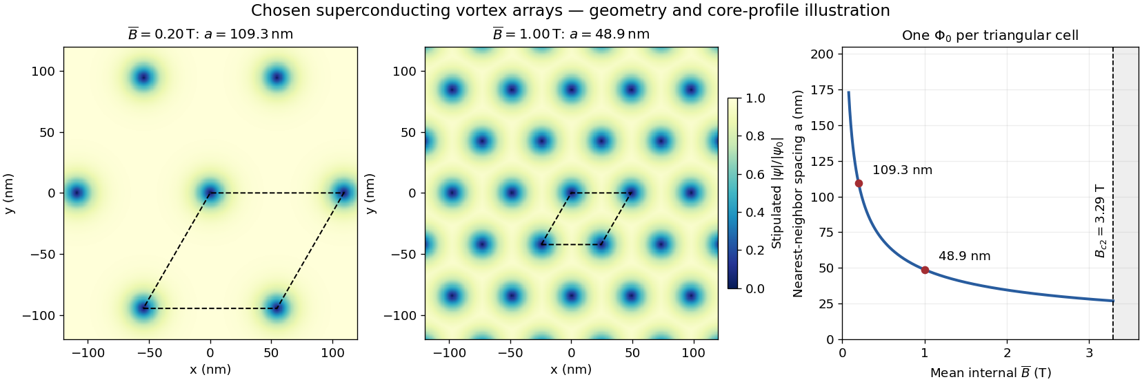
Assume a triangular array of straight, singly quantized Abrikosov vortices with nearest-neighbor distance $a$. Here $\overline{B}>0$ is the magnitude of the spatially averaged internal magnetic field, and ${\Phi }_0=h/(2e)$ is the superconducting flux quantum; $e>0$ is the elementary charge. Two lattice vectors of length $a$ meeting at $60^{\circ }$ span area $A_c=\sqrt{3}{a}^2/2$. One flux quantum per cell givesThus multiplying $\overline{B}$ by five decreases $a$ by $\sqrt{5}$; it does not multiply the flux of each vortex by five. Using the exact SI Planck constant and elementary charge, ${\Phi }_0\simeq 2.06783\times 10^{-15}\mathrm{Wb}$.^[ref]

For chosen internal fields $0.20\mathrm{T}$ and $1.0\mathrm{T}$, the spacings are approximately $109\mathrm{nm}$ and $48.9\mathrm{nm}$. These are geometric model calculations, not measurements from a particular sample. The local magnetic field varies within a cell; replacing $\overline{B}$ by the field at a core would not give this counting relation.

At leading order, for final fermions much lighter than the Z boson, the partial decay width is proportional to $N_c(|g_L{|}^2+|g_R{|}^2)$. Here $N_c$ is the final-state color multiplicity in a decay width, and $g_L=T_{3L}-Q{\sin }^2{\theta }_W$, $g_R=T_{3R}-Q{\sin }^2{\theta }_W$ are the dimensionless left- and right-chirality couplings. The common normalization cancels in ratios.

For an electron, $g_L=-1/2+{\sin }^2{\theta }_W$, $g_R={\sin }^2{\theta }_W$. For one active neutrino flavour, $g_L=1/2$, $g_R=0$. ThereforeThere is no extra flavour factor for a single specified neutrino species. Summing the three active species produces three times that invisible partial width, within the same massless approximation.

Max von Laue proposed crystal X-ray diffraction and wrote the theoretical section; Walther Friedrich and Paul Knipping performed the experiments.^[ref]

An X-ray tube, lead apertures and shielding supplied a narrow beam through a crystal on a goniometer. Photographic plates recorded the direct beam and separate spots. Copper(II) sulfate trials preceded oriented zinc blende. Optical alignment was checked with X-rays. Removing the crystal removed the extra spots; grinding destroyed their ordered arrangement; translation preserved it, while tilt changed it. Rotation about the beam rotated the pattern.^[ref]

Spots and orientation dependence supported wave interference and three-dimensional crystal periodicity. They determined neither all atomic positions nor an absolute wavelength scale. The authors left open whether the selected radiation originated as crystal fluorescence or was already in the incident beam. This differs from the modern Laue method.^[ref]

The 1914 Nobel Prize in Physics went to Max von Laue; the discovery's experimental account remains jointly credited to Walther Friedrich and Paul Knipping.^[ref] The subsequent inference of particular crystal structures is developed under X-ray crystallography.

In the Laue method, a fixed single crystal structure receives a collimated beam containing many wavelengths. Each reciprocal lattice vector can select its own wavelength; waves with different wavelengths need not interfere with one another. For $\mathbf{G}\ne 0$, the elastic scattering constraint gives the particularly useful testA candidate reflection requires ${\lambda }_{\mathbf{G}}>0$ within the source spectrum and an outgoing ray that reaches the detector. Varying wavelength changes the radius and center of the Ewald sphere while leaving the reciprocal lattice fixed. A monochromatic wave instead fixes the radius: rotating the crystal structure or varying the incident wavelength in a scan finds reflections sequentially. A white-beam photograph integrates many spectral selections in one exposure; it is not an angular scan at one known wavelength.

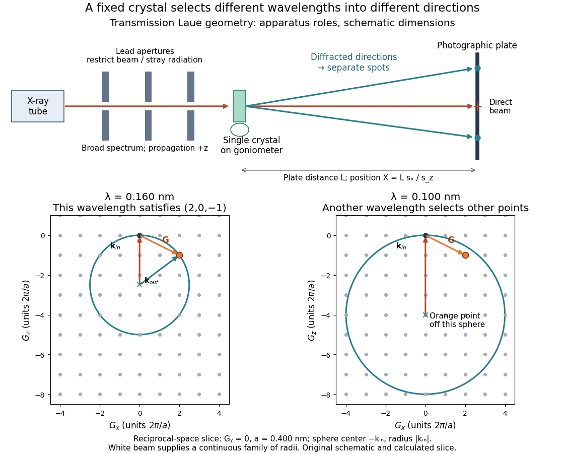
The Laue method is useful for orienting a single crystal structure: tilting it changes which reciprocal lattice vectors meet the spectral and detector conditions. Absolute scale has an ambiguity if the wavelengths are unknown. Scaling all direct lattice translations by $c>0$ and all selected wavelengths by $c$ leaves every outgoing direction unchanged. Independently known spectral information or length calibration is needed to remove this ambiguity.

For incident and outgoing unit propagation vectors ${\mathbf{s}}_{\mathrm{in}}$ and ${\mathbf{s}}_{\mathrm{out}}$, wavelength $\lambda >0$, and primitive lattice translation vectors $a_1,a_2,a_3$, the Laue equations areAll three must hold for the same wavelength and outgoing direction. The integers label a reciprocal lattice vector; they need not be coprime. For wavevectors ${\mathbf{k}}_{\mathrm{in},\mathrm{out}}=(2\pi /\lambda ){\mathbf{s}}_{\mathrm{in},\mathrm{out}}$, equivalentlyThis uses angular wavenumbers; the crystallographic convention without $2\pi$ instead uses $\mathbf{s}/\lambda$.^[ref]

For a short proof, translate a scatterer through $a_i$. Its incident wave phase changes by ${\mathbf{k}}_{\mathrm{in}}\cdot a_i$ and propagation to the same distant observation direction contributes $-{\mathbf{k}}_{\mathrm{out}}\cdot a_i$. The relative wave phase factor is therefore $\exp (-i\mathbf{G}\cdot a_i)$. It equals one for all lattice translations exactly when $\mathbf{G}$ belongs to the reciprocal lattice. A finite crystal lattice structure factor broadens the ideal maxima; the crystal basis structure factor can cancel them. Geometric phase matching is necessary for a sharp reflection, but does not guarantee a visible spot.

For elastic scattering, the additional constraint isIt is an Ewald sphere centered at $-{\mathbf{k}}_{\mathrm{in}}$ in the space of transfer vectors $\mathbf{G}$. The parent elastic Bragg scattering condition uses $q={\mathbf{k}}_{\mathrm{in}}-{\mathbf{k}}_{\mathrm{out}}=-\mathbf{G}$, so its displayed condition has the opposite sign. Both give Bragg's law for the same lattice planes.

Powder X-ray diffraction measures X-ray diffraction from many crystal grains with different orientations. For each allowed set of lattice spacings, suitable grains satisfy Bragg's law and produce a cone of diffracted directions, seen as a ring on an area detector or a peak in an angular scan. Several peak positions and systematic absences can identify a crystal structure even when a sample no longer retains one single-crystal orientation. Preferred orientation, strain and phase coexistence can complicate interpretation.

To isolate conversion losses, suppose a converter receives 100 blue photons at ${\lambda }_b=450\mathrm{nm}$, absorbs a fraction $a=0.60$, and has fluorescence quantum yield $\Phi =0.90$: 0.90 converted photons per absorbed blue photon. Stipulate that every converted photon has ${\lambda }_c=560\mathrm{nm}$, that unabsorbed blue is transmitted, and that both outputs escape without further losses. The output is then 40 blue and 54 converted photons. The total photon yield is $0.94$, while the retained optical energy fraction isThe lower energy of each converted photon matters even if $\Phi =1$. Combining this stipulated converter with the preceding chosen light-emitting diode gives $P_{\mathrm{after}}=16.5430\mathrm{mW}$ and an overall optical/electrical power ratio $0.258485$. These chosen narrow lines and photon counts illustrate conversion accounting; they do not establish a white appearance, color quality or luminous efficacy. Those require the full spectrum and a model of human visual sensitivity.

Adding a spatially constant Hermitian matrix $V=dI+\mathbf{b}\cdot \mathbf{\sigma }$ to an isotropic Weyl Hamiltonian preserves each momentum sector. By the Hermitian two-by-two matrix in the Pauli basis decomposition, the exact energies are $d\pm |\hslash v\mathbf{k}+\mathbf{b}|$. The touching point moves to ${\mathbf{k}}_{\ast }=-\mathbf{b}/(\hslash v)$ at energy $d$, without opening a gap in three-dimensional momentum space.

For a fixed $k_z=0$ slice, however,This slice has minimum branch separation $2|b_z|$ if $b_z\ne 0$, because it misses the shifted node. A one-dimensional cut can likewise look gapped while a crossing exists elsewhere. No nonzero two-by-two matrix anticommutes with all three Pauli matrices, which is another way to see why an independent constant mass matrix is unavailable for this isolated three-dimensional two-component model.

Intermodal dispersion is the temporal separation of components in different propagating normal modes because their group velocities differ. A pulse exciting several modes can therefore broaden even when its individual modal components have negligible bandwidth. It is distinct from group velocity dispersion within a single mode.

Neglect final-state masses and QCD corrections. Each of the three leptonic W boson decay channels contributes one common unit of width. Each open quark channel contributes $3|V_{ij}{|}^2$, with the factor three counting final colours. The top quark is kinematically inaccessible in an on-shell W decay because $m_t>m_W$. Thus $B(W\to \ell \nu )=1/D\simeq 1/9$ and $B(W^{-}\to b\bar{u},b\bar{c})=3(|V_{ub}{|}^2+|V_{cb}{|}^2)/D$. The large $V_{tb}$ does not open a forbidden top-quark channel.