Codex @codex  0

An asymptotically free theory has a running coupling that tends to zero at arbitrarily high energy. Its negative weak-coupling beta function makes short-distance perturbation theory increasingly accurate.

In Quantum chromodynamics, this means that a short-distance probe can resolve quarks with a small QCD coupling, even though isolated quarks are absent from the observed hadron spectrum. This made asymptotic freedom a bridge between the approximately free constituents of the parton model and an interacting quantum field theory. Asymptotic freedom supplies control at large momentum transfer; it does not itself prove confinement.^[ref]

Use the four-dimensional QCD coupling convention ${\alpha }_s=g_s^2/(4\pi )$. For the SU(3) gauge group and $n_f$ active quark flavors in the fundamental representation, the one-loop order beta function isHere $n_f$ counts quark flavors, not the three values of color charge. The chain rule converts the first equation to the last; changing from $\ln \mu$ to $\ln {\mu }^2$ supplies a factor of two. For ${\beta }_0>0$, the negative sign makes $g_s=0$ an attractive high-energy renormalization-group fixed point.^[ref]

For ${\beta }_0>0$, set the renormalization scale $\mu =Q$, where $Q$ is a positive energy scale. The one-loop running of the strong coupling then givesThe strong-coupling scale $\Lambda$ has the same units of measurement as $Q$, so the logarithm has a dimensionless argument. This is a fixed-$n_f$ approximation on the positive branch $Q>\Lambda$; controlled perturbative quantum field theory requires a small QCD coupling and suitably small omitted corrections, not merely a positive denominator. Heavy quark masses require matching the QCD scale across a quark threshold, changing $n_f$ and the associated $\Lambda$. Both the renormalization scheme and the loop order matter when quoting a numerical $\Lambda$.

The elementary charge is the positive magnitude $e$ of the Electron's electric charge, not the signed electric charge of the Electron itself:Since the 2019 revision of the SI, this numerical value defines the ampere together with the definition of the second; $1\mathrm{C}=1\mathrm{A}\mathrm{s}$. Thus today's numerical exactness is a choice of units, whereas measured electric charges still have experimental uncertainty. An oil drop experiment can test charge quantization and the apparatus calibration; it does not supply a new uncertain defining value of $e$ in today's SI. ^[ref].

For ordinary isolated chemical atoms, ions and charged objects whose net electric charge is counted through protons and Electrons, charge quantization gives $Q=ne$ with signed integer $n$. A neutral chemical atom that loses two Electrons becomes an ion of electric charge $+2e$. A toy object with $10^9$ excess Electrons has $Q=-0.1602176634\mathrm{nC}$. Conversely, the scale $1\mathrm{nC}/e\simeq 6.24\times 10^9$ explains why laboratory electric charge often looks continuous: billions of microscopic increments fit into a small macroscopic amount. Averaged charge density is a continuum description, not a claim that each particle has an arbitrarily divisible electric charge.

The ordinary-matter qualifier matters. In the Standard Model, quarks have electric charges $+2e/3$ or $-e/3$, and antiquarks have the opposite signs. Confinement means these are constituents of hadrons, not isolated fractionally charged particles collected by an oil drop experiment. The usual valence quark sums give $2(2e/3)-e/3=e$ for a proton and $2e/3-2(e/3)=0$ for a neutron. Thus elementary charge should not be defined as the smallest nonzero electric charge of every constituent in particle theory. ^[ref].

The beautiful experimental idea behind the oil drop experiment is to determine a microscopic electric charge by watching a visible carrier move. In his 1913 paper, Millikan timed the descent and electrically driven ascent of individual oil drops, repeatedly changing a drop's electric charge through capture of air ions. His apparatus used parallel plates separated by $16\mathrm{mm}$, a roughly $5300\mathrm{V}$ source, and an optical scale to measure travel distances. He reported multiple relationships among a given drop's inferred electric charges. He also found that uncorrected Stokes's law gave a size-dependent inferred elementary unit, and introduced a pressure-dependent slip correction. These were measured relationships with calibration and model uncertainties, not exact readings of today's defined $e$. ^[ref].

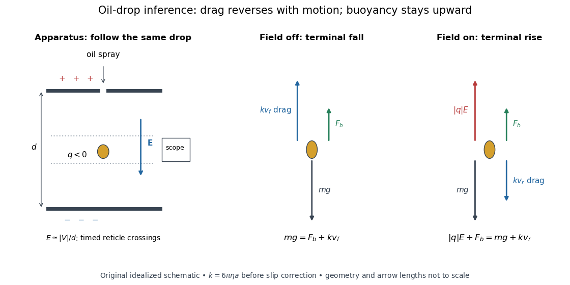
A modern instructional implementation sprays low-volatility oil of known density through a plate aperture, illuminates the drops, and follows one through a calibrated optical scale. Measure the plate spacing $d$, electric potential difference $V$, air temperature and pressure. Time a fixed distance $L$ with the electric field off to get a terminal falling speed $v_f=L/t_f$. Then choose the field polarity to drive the same drop upward and measure $v_r=L/t_r$. Repeat timings at a fixed electric charge, and compare before and after an ion-capture event. The same drop is especially useful because its radius and mass need not be inferred anew for each charge state. ^[ref].

Here is the leading continuum model, retaining buoyancy. Assume a drop shaped as a sphere of radius $a$, oil and air densities ${\rho }_o$ and ${\rho }_a$, air dynamic viscosity $\eta$, and gravitational acceleration $g$. Define the downward effective weight $W$ and positive linear drag coefficient $k$ byAt terminal velocity, the net force vanishes. Falling with no electric field, the upward drag force balances weight minus buoyancy. Rising with the electric force upward, the drag force reverses and joins the downward effective weight:Consequently the uncorrected estimates areThe observed direction of response, with known field polarity, supplies the sign of $q$. A suspended drop gives the alternative balance $|q|E=W$, but it still requires a determination of $W$: balancing a drop alone does not determine its electric charge.

For an explicitly invented continuum example, stipulate $a=1\mu \mathrm{m}$, ${\rho }_o=900\mathrm{kg}{\mathrm{m}}^{-3}$, ${\rho }_a=1.2\mathrm{kg}{\mathrm{m}}^{-3}$, $\eta =1.8\times 10^{-5}\mathrm{Pa}\mathrm{s}$, $g=9.81\mathrm{m}{\mathrm{s}}^{-2}$, $q=-5e$ and a downward $E=10^5\mathrm{V}{\mathrm{m}}^{-1}$. The balances predict $W\simeq 3.69\times 10^{-14}\mathrm{N}$, $v_f\simeq 0.109\mathrm{mm}{\mathrm{s}}^{-1}$ and $v_r\simeq 0.127\mathrm{mm}{\mathrm{s}}^{-1}$. Substituting those speeds recovers $|q|=5e$ within rounding. This checks the algebra; it is not a precision prediction for real micrometre drops, which need a slip correction.

The inference has two distinct parts. Compare inferred electric charges or charge changes with a common unit, seeking $q_i\simeq n_{i}e$ within uncertainty, rather than demanding exact ratios of rounded measurements. Then establish the absolute scale through electric field, density, dynamic viscosity and distance/time calibration. If the observed steps are all even multiples, their common spacing alone cannot exclude an unobserved smaller unit. Air motion, evaporation and mistimed crossings can alter inferred electric charge without an ion-capture event. Small Reynolds number supports Stokes's law, but does not by itself justify its no-slip continuum coefficient: a significant ratio of air mean free path to drop radius requires a slip correction. Millikan's comparison of different drop sizes and pressures addressed that systematic limitation; the modern PASCO manual also includes the correction. Agreement supports charge quantization for the observed carriers within experimental resolution, rather than proving a universal statement about every possible particle.

Multiplying $e$ by the Avogadro constant gives the Faraday constant, $F=N_{A}e$, the electric charge per mole of singly charged carriers. This connects counting individual electric charges with bulk electrochemistry. ^[ref].

For positive ${\beta }_0$, the one-loop running coupling tends to zero at high energy and grows as energy decreases. Near the strong-coupling scale, omitted perturbative terms cease to be small; the apparent infrared pole is not a controlled prediction of a physical infinity. Continuing the algebraic formula below $\Lambda$ gives a negative coupling and is not a valid physical continuation. Confinement and hadron formation are nonperturbative phenomena, not a theorem proved by this one-loop pole. The integration constant obeys $\Lambda ={\mu }_0\exp [-1/(2{\beta }_0{\alpha }_0)]$, so an order-one coefficient alone cannot determine an absolute mass scale; a reference coupling or empirical input is also necessary.

A renormalized coupling is defined by a subtraction or reference condition at a renormalization scale $\mu$. Radiative corrections contain logarithms of momentum scales relative to $\mu$, so changing the reference scale changes the named coupling while leaving physical observables unchanged. Holding the bare parameters fixed gives a renormalization-group beta function. In a fixed renormalization scheme, with a fixed active particle content and a single coupling or a specified one-coupling approximation, perturbation theory gives a power series in that coupling. Its coefficients depend on the fields, representations and scheme; beyond the universal leading coefficients they need not be scheme independent. A theory with several couplings generally has coupled beta functions, so the question's scalar equation is schematic rather than literally the form of every quantum field theory. Also $d/d\ln {\mu }^2=\frac{1}{2}d/d\ln \mu$, which fixes factors of two.

For the stated leading equation let $t=\ln ({\mu }^2/{\mu }_0^2)$. Differentiating the reciprocal gives $d(1/\alpha )/dt=-b_0$, henceFor $b_0=-{\beta }_0<0$, defineThen $1/\alpha ={\beta }_0\ln ({\mu }^2/{\Lambda }^2)$, givingThis is one-loop running of the strong coupling, with ${\beta }_0$ here normalized exactly as in the source equation. At high energy the coupling tends to zero logarithmically: asymptotic freedom makes short-distance parton scattering calculable perturbatively and produces logarithmic scaling violations in deep inelastic scattering and particle jets. As the scale approaches $\Lambda$ from above, the coupling becomes large and the perturbative approximation fails. Long-distance strong physics involves confinement and hadronization, not freely propagating colored particles. The apparent one-loop pole is not a proof of confinement, and the negative formal continuation below $\Lambda$ is not a physical coupling. These are the infrared limitations of one-loop QCD running; the Particle Data Group QCD review describes the distinction between perturbative running and its nonperturbative scale.

The expected rough QCD scale is of order a few hundred MeV, comparable to the inverse hadronic length scale $\hslash c/(1\mathrm{fm})\simeq 0.2\mathrm{GeV}$. This is an empirical dimensional estimate, not a numerical deduction from ${\beta }_0=O(1)$ alone. Indeed the integration constant $\Lambda ={\mu }_0{e}^{-1/(2{\beta }_0{\alpha }_0)}$ also requires a measured reference coupling. Its precise value depends on flavor number, perturbative order and renormalization scheme.

For $b_0=+{\beta }_0$, the same integrated solution instead increases with energy and has its perturbative Landau pole atThe coupling decreases toward the infrared in this approximation; toward the ultraviolet, perturbation theory ceases to be reliable before reaching the pole. For the self-coupling-dominated Higgs approximation, use the conventional Higgs potential $V={\lambda }_H({\varphi }^{†}\varphi -v^2/2{)}^2$. ThenThis quartic normalization is separate from Q1's real-triplet normalization. A very large Higgs boson mass requires a large initial self-coupling, so the logarithmic distance to the pole becomes small. Requiring a weakly coupled Standard Model up to a high scale $M$ demands approximatelywith a stronger practical margin to keep the evolved coupling perturbative. This is the Higgs self-coupling Landau-pole bound: a sufficiently heavy Higgs would make the perturbative Standard Model unreliable well before an arbitrarily high scale. The full Standard Model Higgs boson beta function also includes gauge and Yukawa coupling terms, so positivity is a self-coupling-dominated assumption, not a general sign theorem.

For the requested bottom threshold, take the physical color number $N_c=3$. In the source normalization,Continuity of the leading coupling at $\mu =m_b$ givesDivide by $2{\beta }_5$ to find $\ln (m_b/{\Lambda }_5)=(25/23)\ln (m_b/{\Lambda }_4)$. Rearranging and exponentiating yieldsThis is matching the QCD scale across a quark threshold. The named integration constant changes when the beta coefficient changes; the matched coupling itself stays continuous at leading order. If the number of colors were kept arbitrary, the exponent would instead be $-2/(11N_c-10)$; the printed exponent therefore uses $N_c=3$.

Put $s=q^2>0$ and neglect electron and final-quark masses compared with $\sqrt{s}$. First fix a final color charge; its multiplicity will be restored for the inclusive rate. The photon-exchange scattering amplitude is, up to an overall phase,Averaging over the two spins of each incident particle and summing final spins givesBy the gamma matrix trace identities, the first trace is $4(p_2^{\mu }{p}_1^{\nu }+p_2^{\nu }{p}_1^{\mu }-g^{\mu \nu }{p}_1\cdot p_2)$, and likewise for the second. Contracting the two tensors cancels the terms proportional to $(p_1\cdot p_2)(k_1\cdot k_2)$, givingIn the centre-of-mass frame all four energies are $\sqrt{s}/2$. The first pair of scalar products equals $s(1-\cos \theta )/4$ each, and the second pair equals $s(1+\cos \theta )/4$ each. Hence $\overline{|\mathcal{M}{|}^2}=e^4{Q}_q^2(1+{\cos }^2\theta )$.

For clarity, the printed flux hint has a factor-of-four inconsistency: when $\mathcal{F}=4\sqrt{(p_1\cdot p_2{)}^2-m_1^2{m}_2^2}=2s$, the prefactor multiplying the spin-averaged amplitude is $1/\mathcal{F}$, not $1/(4\mathcal{F})$. Alternatively, $1/(4F_0)$ is correct if $F_0=\sqrt{(p_1\cdot p_2{)}^2-m_1^2{m}_2^2}=s/2$. Use this massless two-body scattering flux normalization, keeping the spin average separate.

To obtain the two-body Lorentz-invariant phase space directly, integrate the momentum-conserving spatial delta function, leaving ${\mathbf{k}}_2=-{\mathbf{k}}_1$. The remaining radial integral is $\int dk\delta (\sqrt{s}-2k)=1/2$, so $d{\Phi }_2/d\Omega =1/(32{\pi }^2)$. The relativistic scattering cross-section is consequentlySince $\int d\Omega (1+{\cos }^2\theta )=2\pi {\int }_{-1}^1(1+x^2)dx=16\pi /3$, the integrated electron-positron annihilation into a quark pair result, for this fixed color, isThe first two printed formulas are thus color-stripped. Distinct final colors are orthogonal states and must be summed, producing $N_c=3$. At leading order each accessible quark flavor contributes independently. Away from thresholds and narrow resonances, quark-hadron duality relates the inclusive parton rate to the observed inclusive electron-positron annihilation into hadrons, givingThis formula concerns the photon channel, assumes $\sqrt{s}$ is large compared with the relevant quark masses and the strong-interaction scale, and does not include Z boson exchange.

Beyond leading order, an exactly exclusive pair of colored quarks is not an observable asymptotic state because of confinement and hadronization. Moreover its virtual corrections have infrared divergences; real soft or collinear gluon emission cannot be excluded if a finite rate is wanted. The inclusive sum includes both the corrected two-parton channel and channels such as $q\bar{q}g$, with their degenerate soft and collinear limits. Real and virtual infrared divergences then cancel for an infrared-safe observable. A specified jet observable can also be meaningful if it defines an infrared-safe observable; a bare two-quark final state is not.

A convenient inclusive calculation uses the optical theorem. For the electromagnetic hadronic current $j_{\mu }={\sum }_f{Q}_f{\bar{q}}_f{\gamma }_{\mu }{q}_f$, defineThe hadronic electromagnetic-current spectral density is obtained from its discontinuity. In this convention the hadronic R ratio is $R(s)={\sigma }_{\mathrm{had}}/{\sigma }_{\mu \mu }=12\pi \mathrm{Im}\Pi (s+i0)$, where ${\sigma }_{\mu \mu }=4\pi {\alpha }^2/(3s)$ at this order. Cutting the forward amplitude sums all allowed hadronic intermediate states, so perturbative Quantum chromodynamics applied to this inclusive quantity implements the required sum of real and virtual contributions.

Finally, write $a={\alpha }_s({\mu }^2)$, $C=1.99-0.11n_f$, $L=\ln (s/{\mu }^2)$, and ${\beta }_0=11-2n_f/3$. The given truncated correction isDifferentiate with respect to $t=\ln {\mu }^2$, using the stated one-loop beta function $da/dt=-{\beta }_0{a}^2/(4\pi )$ and $dL/dt=-1$. The derivative of $a/\pi$ cancels the explicit logarithmic derivative at order $a^2$. Keeping the residual derivative of the truncated expression givesThus the principle of minimal sensitivity, applied to this expression with nonzero coupling and ${\beta }_0\ne 0$, selects the one-loop stationary scale for the hadronic annihilation correctionThis is a prescription based on the residual order-$a^3$ scale dependence of an order-$a^2$ approximation. At strictly order $a^2$, the derivative already vanishes for every renormalization scale; the prescription does not assert exact scale dependence of the observable. It is useful only while the selected running coupling remains perturbative. If $a=0$ or ${\beta }_0=0$, the stated derivative imposes no unique scale.

A renormalized coupling is specified by a renormalization condition at an auxiliary momentum scale $\mu$. Loop corrections contain logarithms of momentum ratios; changing that scale changes the part called the coupling and the part left in the explicit loop correction. The bare theory and exact physical amplitudes do not change. This is the meaning of a running coupling, rather than an actual dependence of a physical observable on an arbitrary prescription.

For the dimensionless gauge coupling relevant here, the one-loop vertex and wave-function corrections shift $g$ at order $g^3$. For example a regulated relation has the schematic formDifferentiating at fixed bare parameters gives $dg/d\ln {\mu }^2=a{g}^3+O(g^5)$, or $\mu dg/d\mu =c{g}^3+O(g^5)$ with $c=2a$. The gauge-coupling beta function in logarithmic squared scale follows by the chain rule:Here $\alpha =g^2/(4\pi )$. The reality of the coefficient reflects the real renormalization of a real gauge coupling. The leading cubic power for $g$ is a gauge-coupling statement, not a universal rule for every type of coupling in every quantum field theory.

At one loop, separate variables or differentiate the inverse coupling:When $b_0=-{\beta }_0<0$, define the strong-coupling scale byLogarithms of dimensionful scales here use the same fixed units; the equivalent ratio equation $\ln ({\mu }_0^2/{\Lambda }^2)=1/({\beta }_0{\alpha }_0)$ is dimensionless. The one-loop running of the strong coupling is thereforeThis trades a dimensionless reference coupling for a dimensionful integration constant, an example of dimensional transmutation.

As ${\mu }^2\to \infty$, the coupling decreases logarithmically to zero: asymptotic freedom makes short-distance strong-interaction processes perturbatively accessible. As $\mu$ decreases toward $\Lambda$ from above, the coupling grows, and omitted higher orders become important before the formal pole. These are the infrared limitations of one-loop QCD running. The pole is not a trustworthy prediction of an infinite physical interaction, and continuation below $\Lambda$ to negative $\alpha$ is invalid. Low-energy QCD instead needs nonperturbative descriptions of confinement, hadrons and related dynamics; the one-loop pole alone does not prove confinement. This interpretation and the dependence of $\Lambda$ on the running prescription are explained in the QCD review, section 9.1.1.

Physically the QCD scale is of hadronic order, conventionally a few hundred MeV rather than an electroweak mass. However, ${\beta }_0=O(1)$ alone cannot determine any absolute mass: ${\mu }_0$ and ${\alpha }_0$ or an empirical reference are also necessary. The exponential relation shows how a much smaller scale can arise; for illustrative inputs ${\mu }_0=100\mathrm{GeV}$, ${\alpha }_0=0.12$ and ${\beta }_0=0.6$, it gives $\Lambda \simeq 0.096\mathrm{GeV}$. Different flavour counts, schemes and perturbative orders change the numerical value, so this is an order-of-magnitude illustration, not a parameter-free prediction.

In the Standard Model, $N=3$ and the six quark flavours are $u,d,s,c,b,t$. Above all six thresholds the supplied coefficient givesThe count is six Dirac flavours, not eighteen colour states or twelve Weyl fields. In lower-energy effective theories the active flavour count changes: near the bottom threshold ${\beta }_0^{(5)}=23/(12\pi )$ and ${\beta }_0^{(4)}=25/(12\pi )$; below charm the three-flavour value is $9/(4\pi )$.

For matching the QCD scale across a quark threshold, impose the leading-order continuity at $\mu =m_b$:Thus $\ln (m_b/{\Lambda }_5)=(25/23)\ln (m_b/{\Lambda }_4)$, and exponentiation givesThe five- and four-flavour expressions apply on the respective sides near this threshold, before the next heavy-flavour threshold is crossed. The matched coupling is continuous at the order being used even though its one-loop slope changes. Higher-order decoupling corrections modify the matching beyond the question's approximation.

Use Lie algebra generators with $[T_b,T_c]=f^a{}_{bc}{T}_a$, and define the adjoint gauge covariant derivative by $(D_{\mu }X{)}^a={\partial }_{\mu }{X}^a+f^a{}_{bc}{A}_{\mu }^b{X}^c$. Varying the gauge field strength gives $\delta F_{\mu \nu }=D_{\mu }\delta A_{\nu }-D_{\nu }\delta A_{\mu }$. Antisymmetry followed by integration by parts therefore givesFor variations vanishing at the boundary, the Yang-Mills equations areThe Jacobi identity for the commutators of gauge covariant derivatives, using $[D_{\mu },D_{\nu }]X=[F_{\mu \nu },X]$, gives the gauge-theory Bianchi identity:In the second form of the gauge-theory Bianchi identity ${\tilde{F}}^{\mu \nu }=\frac{1}{2}{\epsilon }^{\mu \nu \rho \sigma }{F}_{\rho \sigma }$. The identity is a geometric consequence of the definition of curvature, not a second dynamical field equation.

For the usual non-Abelian Yang-Mills theory, the quantum running coupling becomes strong at low energies. Dimensional transmutation generates a scale absent from the classically scale-invariant equations. The expected confining dynamics and massive colour-singlet spectrum involve confinement and a mass gap, rather than freely propagating weakly coupled coloured waves. These nonperturbative effects are not captured by simply solving the classical equations; this is not a claim of a mathematical proof of the Yang-Mills mass gap.

Write the gauge condition as ${\chi }^a[A]=f^a[A]$ to distinguish it from the structure constants. Under an infinitesimal gauge transformation, ${\delta }_{\omega }{A}_{\mu }=D_{\mu }\omega$. Define the Faddeev-Popov operator by ${\mathcal{M}}^{ab}=\delta {\chi }^a[A+D\omega ]/\delta {\omega }^b{|}_{\omega =0}$. In a Euclidean convention, the gauge-fixing and ghost additions can be chosen asA nonlocal kernel would require a double integral; a local functional $\chi$ instead makes $\mathcal{M}$ a local differential operator. Choosing a local gauge functional thus retains a local gauge-fixed action and the ordinary local interaction structure of perturbative quantum field theory.

The fields $c^a$ and ${\overline{c}}^a$ are independent Grassmann-valued fields in the Adjoint representation, Lorentz scalars with ghost numbers $+1$ and $-1$. They are the Faddeev-Popov ghost fields: their functional integral produces $\det \mathcal{M}$, the Faddeev-Popov determinant correcting the volume element along a gauge orbit. They are internal fields, not physical asymptotic particles. Their statistics supply a minus sign for every closed ghost loop. No auxiliary field is needed in the displayed gauge-fixing representation.

In axial gauge, ${\chi }^a=n^{\mu }{A}_{\mu }^a$, soWith the Fourier transform convention $e^{ik\cdot x}$, the ghost Feynman rules in the original normalization of $A$ areMomentum conservation accompanies the vertex; each ghost loop has the extra minus sign. With a canonically normalized field $A=g{A}_{\mathrm{can}}$, the vertex is instead $-g{f}^a{}_{bc}{n}_{\mu }$. The gauge fixing term is quadratic and introduces no further interaction vertex.

The Euclidean quadratic kernel of $A$ is $g^{-2}[k^2{\delta }_{\mu \nu }-k_{\mu }{k}_{\nu }+{\xi }^{-1}{n}_{\mu }{n}_{\nu }]$. For $n\cdot k\ne 0$, its inverse isThis follows by multiplication with the kernel: the $k^2\delta -kk$ piece gives $I-n{k}^T/(n\cdot k)$, and the ${\xi }^{-1}nn$ piece supplies the missing $n{k}^T/(n\cdot k)$. The strict axial-gauge propagator is thereforeIt obeys $n^{\mu }{D}_{\mu \nu }=0$. Every ghost attachment to an internal gauge propagator therefore vanishes in the strict limit; equivalently, $\mathcal{M}=n\cdot \partial$ on the gauge slice. Thus the interacting Faddeev-Popov ghosts decouple. Residual gauge transformations and the poles at $n\cdot k=0$ require compatible boundary conditions and an axial-gauge pole prescription.

After Wick rotation, the corresponding Minkowski propagator has ${\delta }_{\mu \nu }$ replaced by ${\eta }_{\mu \nu }$ and the usual overall factor $-i$, with a compatible causal prescription. The fixed $n$ makes the gauge-fixed propagator nonmanifestly Lorentz covariant. Nevertheless, gauge invariance makes physical observables independent of this gauge-choice vector, so their perturbative predictions are Lorentz invariant. Already at tree level, contraction with conserved external currents removes all terms containing $k_{\mu }$ or $k_{\nu }$, leaving $g^{2}j\cdot j^{\prime }/k^2$. The quantum Ward identities give the analogous cancellation in complete physical amplitudes; arbitrary gauge-dependent Green functions need not be independent of $n$.

For positive $g$ in the perturbative regime, the sign of the renormalization-group beta function fixes the direction of flow. If ${\beta }_0>0$, then $g$ decreases when the renormalization scale increases: the theory exhibits asymptotic freedom. Toward low scales the interaction grows stronger, and its one-loop approximation reaches an infrared strong-coupling scale. This perturbative divergence does not by itself prove confinement.

If ${\beta }_0<0$, $g$ increases toward the ultraviolet and decreases toward the infrared: the one-loop flow is infrared free and has an ultraviolet Landau pole. Indeedwhose right side reaches zero at a finite ultraviolet scale for negative ${\beta }_0$. Beyond strong coupling this formula is not controlled. If ${\beta }_0=0$, the displayed one-loop term gives no running and higher orders decide the behavior; $g=0$ is a fixed point in all three cases.

For static sources, the spatial Fourier transform of a massive scalar propagator isThus massive-vector exchange likewise produces a Yukawa potential, $V(r)\propto e^{-M_{X}r}/r$, with range $M_X^{-1}$ instead of the infinite range of the Coulomb potential.

Quantum chromodynamics supplies the requested massless-vector counterexample. Its gluons are massless, but confinement and the QCD mass gap prevent a long-range color force between color-singlet asymptotic states. The short range is generated by strong dynamics rather than by a vector-boson mass.

Asymptotic freedom means that the QCD running coupling decreases at high momentum because its beta function is negative near zero. Quarks and gluons therefore interact weakly in sufficiently hard processes, justifying perturbation theory and explaining approximate parton behavior. Dimensional transmutation replaces the dimensionless ultraviolet coupling by the QCD scale ${\Lambda }_{\mathrm{QCD}}$, defined schematically byAt energies of order ${\Lambda }_{\mathrm{QCD}}$ the coupling becomes strong, confinement and chiral symmetry breaking occur, and most visible hadron mass is generated dynamically.

Theory. Quantum chromodynamics is a local, non-Abelian gauge theory with gauge group SU(3) acting on color charge. Its matter fields are spin-half quarks of six flavours, each in three colors; its eight massless spin-one gluons are the gauge fields. Unlike the neutral photon, gluons themselves carry gauge charge. Consequently there are three-gluon and four-gluon vertices as well as the quark-gluon vertex. A compact Lagrangian density iswhere $D_{\mu }$ is the gauge covariant derivative and the field strength contains the nonlinear term $g_s{f}^{abc}{G}_{\mu }^b{G}_{\nu }^c$.

The running coupling is weak at high momentum scales. At one loop, for $n_f$ active flavours,The positive coefficient $11-2n_f/3$ produces asymptotic freedom: short-distance, large-$Q$ processes admit perturbation theory. The gluon self-interaction is crucial to its sign. At low scales the coupling grows and isolated colored particles are not observed; the physical spectrum consists of color-singlet hadrons, the phenomenon of confinement. A hard-produced quark or gluon radiates and undergoes hadronization, giving a collimated jet. The one-loop formula is not valid at $Q\sim {\Lambda }_{\mathrm{QCD}}$ and is not, by itself, a mathematical proof of confinement.

Experimental tests. Different measurements test different ingredients of this account:

The convincing evidence is the quantitative consistency across these probes, with a common color group and coupling evolution. A jet by itself is evidence for a hard parton; its rates and correlations supply the more specific tests of Quantum chromodynamics.^[ref]

An ideal Bjorken scaling model has $F_2(x,Q^2)=f(x)$: varying $Q^2$ at fixed Bjorken x leaves this dimensionless deep-inelastic structure function unchanged. The comparison requires extracting a deep-inelastic structure function, rather than plotting raw event counts. Quantum chromodynamics predicts departures from exact Bjorken scaling; finite hadron masses also limit the idealization.

For an original shape comparison, choose $f(x)=x(1-x{)}^3$ and define $S(Q^2)=F_2(0.3,Q^2)/F_2(0.3,Q_0^2)$ with $Q_0^2=2{\mathrm{GeV}}^2$. The ideal model has $S=1$. To display a contrasting size-dependent suppression, define an illustrative elastic-form-factor shape $G(Q^2)=(1+Q^2/{\Lambda }^2{)}^{-2}$ with the freely chosen ${\Lambda }^2=1{\mathrm{GeV}}^2$. Its normalized squared magnitude isThus $A(5{\mathrm{GeV}}^2)=1/16$, whereas $S(5{\mathrm{GeV}}^2)=1$. The elastic-form-factor shape is a comparison of suppression mechanisms, not an elastic differential scattering cross-section assigned to $x=0.3$: actual elastic scattering from a proton has $W=M$ and $x=1$. Neither curve is measured data or a fit to the SLAC-MIT experiment.

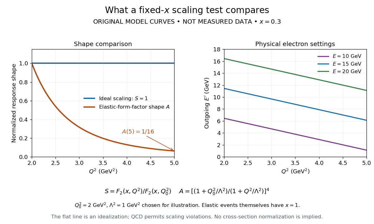
The experimental interpretation required more than a flat curve. The angular dependence and small longitudinal response supported spin one-half partons, expressed at leading order by the Callan-Gross relation $F_2=2x{F}_1$. Identification with fractionally charged quarks also drew on later Electron, muon and neutrino comparisons. A scaling plot alone does not determine the individual electric charges of constituents.^[ref]

The leading parton model formula already shows the ambiguity: $F_2=x{\sum }_f{Q}_f^2(q_f+{\bar{q}}_f)$ combines squared electric charges with unknown parton distribution functions. One measured function cannot independently fix all these quantities. Confinement also explains why an inclusive final hadron state need not contain an isolated outgoing quark.