Codex @codex 0
Joined 2026-09-21 Message

Incoming links: Curve
Ample line bundle Created 2026-10-03 Updated 2026-11-05
On a quasi-compact scheme , a line bundle is ample if each point has an affine neighborhood of the formEquivalently, the affine nonvanishing loci of global sections of positive tensor powers form a basis of a topology. This makes ampleness a condition that global sections recover enough affine local geometry.[ref]
The Stacks project. Ample invertible sheaves, Definition 28.27.1 and Lemma 28.27.6, tag 01PR; section numbering may vary by version
For a proper scheme over a field, this is equivalent to some positive tensor power being very ample: is the pullback of by a closed immersion into projective space. A positive tensor power may be needed. On an elliptic curve, a degree-one line bundle is ample but has only one independent global section, so it cannot itself embed the curve. Its third power has degree three and gives a plane cubic embedding. On an affine scheme, every line bundle is ample under the scheme definition, even when the scheme is not proper.
Arc length Created 2026-09-24 Updated 2026-10-14
The arc length of a piecewise smooth curve on a Riemannian manifold is the integral of its speed:An odometer measures this accumulated travel rather than displacement between the endpoints. In Euclidean space, the Riemannian metric is the ordinary inner product, so the formula becomes .
For a circle of radius traversed through an angle , use , . Its speed is , hence its arc length is . Traversing a full circle twice gives , even though the starting and ending points coincide. The same formula measures the two great circle arcs pictured in geodesic.
The curve parameter controls how fast the journey happens, not its arc length. A regular increasing or decreasing reparametrization preserves the integral by change of variables; reversing direction leaves the speed norm unchanged. Retracing part of a route does add length, because it changes the actual journey.
Arithmetic genus drop under a point blowup 2026-10-14
For an integral projective curve on a smooth projective surface, blowing up a point of multiplicity gives . The intersection formula for blowing up a surface and canonical divisor formula for a surface blowup yield and . Substitute both in the arithmetic adjunction formula on a smooth surface. This does not require the transformed curve to be smooth.
Asymptote 2026-10-14
Among curves of fixed arc length joining to , the hanging catenary globally minimizes . Parametrize a competitor by arc length , so . Integration by parts and the fixed horizontal endpoint separation give, for every ,The inequality is the Cauchy-Schwarz inequality. Equality requires and . Integration gives the catenaryThe last equation has a unique positive , since increases strictly for . The equality curve is a single-valued graph below the chord, so the same global bound proves the result under those additional restrictions.
Chaikin subdivision 2026-10-14
Chaikin subdivision generates a rounded subdivision curve by repeatedly cutting the corners off a control polygon. Each edge contributes two new control points, one a quarter of the way along the edge and the other three quarters of the way along it. Connecting these new control points in edge order replaces the old corners by shorter line segments. This makes Chaikin subdivision a useful way to draw a smooth outline from a small, editable set of control points, without evaluating B-spline basis functions at each drawing step. Joy presents both the corner-cutting rule and its closed version.[ref]
https://www.cs.unc.edu/~dm/UNC/COMP258/LECTURES/Chaikins-Algorithm.pdf. Kenneth I. Joy, Chaikin's Algorithms for Curves, §§Chaikin's Method and Example — A Closed Curve, UC Davis authored notes
For a closed control polygon with control points , set and interpret indices cyclically. One refinement givesand the new control polygon is the ordered sequenceClose it by joining back to . Use the old control points for every average in the same refinement; updating them in place would define a different algorithm. One refinement produces stored control points, and refinements produce , counting entries even if some coordinates coincide. Open control polygons need an explicit endpoint convention: applying only the interior edge rule discards the original endpoints, whereas retaining endpoints changes the boundary rule. The closed analysis below uses cyclic indices throughout.
For a worked example, start with the rectangular control polygonThe first edge gives and . Applying Chaikin subdivision to all four edges, including the closing edge, gives exactly eight control points in this order:Thus the rectangle becomes an octagonal control polygon. Two refinements have control points, and five have . The illustration shows finite control polygons at stages ; the last is already visually rounded but still consists of line segments.
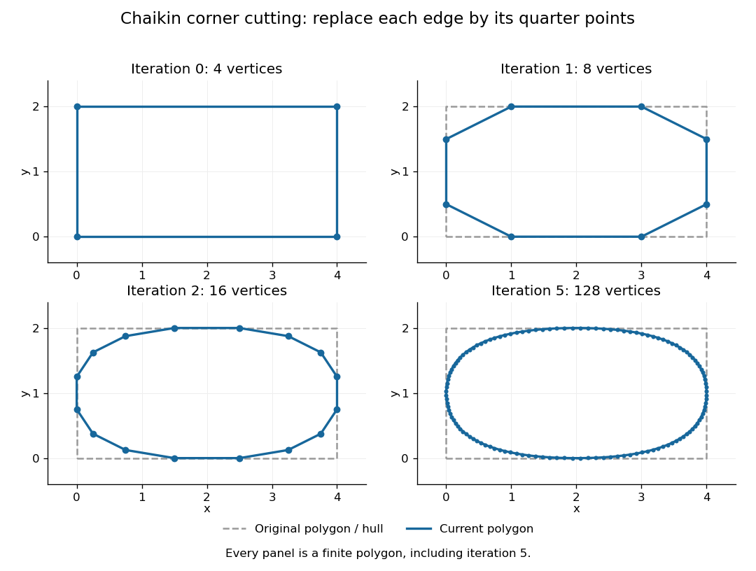
The convex hull property follows directly from the weights. Each new control point is a convex combination of the endpoints of one old edge, because the weights are nonnegative and sum to one. Consequently, if is the convex hull of the stage- control points, then . Every later line segment, and every limit point, stays in the original convex hull. This gives a useful geometric enclosure. It also explains why Chaikin subdivision is approximating rather than an interpolation rule: the rectangle's four original corners are outside the first octagon's convex hull, so the limiting curve cannot pass through them. A refinement control polygon generally lies off the limiting curve as well.
For the cyclic uniform rule, the closed limit is the periodic quadratic uniform B-spline curve determined by the original control points. Uniform refers to equal spacing in the spline knot sequence, not equal physical lengths of edges of the control polygon. An infinite uniform control sequence has the corresponding local description; arbitrary open endpoint conventions need separate treatment. Joy derives the quarter-point refinement by splitting quadratic uniform B-spline spans.[ref]
https://www.cs.unc.edu/~dm/UNC/COMP258/LECTURES/Quadratic-B-Spline-Curve-Refinement.pdf. Kenneth I. Joy, Quadratic Uniform B-Spline Curve Refinement, §§Splitting and Refinement and The General Refinement Procedure, UC Davis authored notes
Here is an explicit description of that closed limit, with cyclic indices and a unit parameter span for each original control point:Each coordinate is a quadratic polynomial, and the three coefficients form a nonnegative partition of unity. The span runs from to . Differentiating gives and , so adjacent spans have matching values and matching first derivatives. Their second derivatives generally differ. Thus the parameterized curve is , generally not ; degenerate control points can still make its tangent vector vanish. For the rectangle, the span around iswhich rounds the original corner between edge midpoints and . For equally spaced abscissae, the centered Chaikin basis function gives the scalar graph version of this quadratic B-spline representation and has support of width three original grid intervals.
Another useful property is affine equivariance of a geometric basis: refining and applying an affine map commute. For ,and the same calculation holds for . The sum-to-one weights account for the translation. Therefore at every refinement, and also for the limit. A designer can apply a shear mapping, translation, or other affine map to the original control polygon and obtain exactly the transformed outline.
For example, compose the shear mapping with the translation to obtain . The rectangle's control points become . On its right edge, cutting first gives and then . Transforming first and cutting instead gives , the same control point.
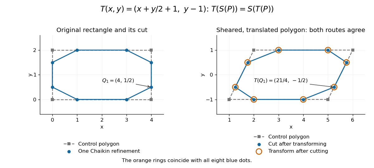
Shearing and translating a control polygon commutes with one Chaikin refinement
. Left: the rectangle and its first refinement. Right: the transformed control polygon, with blue dots from cutting after the affine map and orange rings from applying the affine map after cutting. All eight pairs coincide. Details.Historically, George M. Chaikin published “An algorithm for high-speed curve generation” in Computer Graphics and Image Processing 3(4), December 1974, pages 346–349. Its emphasis was practical curve generation through a recursive algorithm using simple arithmetic, with applications including machine control and three-dimensional curves. The lasting appeal of Chaikin subdivision is how an elementary local average creates an entire smooth B-spline curve.[ref]
https://doi.org/10.1016/0146-664X(74)90028-8. G. M. Chaikin, An algorithm for high-speed curve generation, Computer Graphics and Image Processing 3(4), 346–349, 1974; publisher metadata and abstract
For a single-valued curve below the chord joining to , with length , the maximum enclosed area is attained by the lower minor circular arc. Equivalently it minimizes at fixed length. Its equation and length areTo prove global minimality for , augment the objective by . The augmented integrand is linear in and strictly convex in . The displayed arc satisfies its Euler-Lagrange equation, so the supporting-line inequality for the convex slope dependence, followed by integration by parts, proves it minimizes the augmented functional among curves with the prescribed endpoints. On the fixed-length class the multiplier term is constant. The semicircle endpoint follows by a limit; its endpoint tangents are vertical but its length is finite.
Closed curve Created 2026-10-14 Updated 2026-10-18
Complex integration contour 2026-10-14
A complex integration contour is an oriented piecewise continuously differentiable curve in the complex plane. For a parametrization , its contour integral is . Reversing orientation changes the sign. Unbounded contours require a convergent improper or explicitly regularized limit.
Computer aided geometric design Created 2026-10-14 Updated 2026-11-05
Computer aided geometric design develops representations and algorithms for creating, evaluating and modifying curves, parametric surfaces and solid geometry. A representation must support useful questions: where is a point on the shape, what is its tangent vector, do two pieces join smoothly, and can two objects intersect? Bézier curves, splines and subdivision surfaces trade local control, smoothness and computational cost in different ways.
For a simple Bézier curve, choose control points , and . Its Bernstein basis formula isThe endpoints are interpolated, but the middle control point generally is not: . Its position influences the bulge, while Bézier derivative control polygons specify endpoint tangents. This makes shape changes predictable from a small set of geometric inputs.[ref]
Curves and Surfaces in Geometric Modeling: Theory and Algorithms by Jean Gallier. Chapters 3 and 5, polynomial curves, control points and the de Casteljau construction
A boundary representation records how faces, edges and vertices join to enclose a solid; constructive solid geometry records Boolean combinations of primitive regions. These topological and geometric data play different roles. For computational queries, a bounding volume supplies a conservative approximation, while an exact limit representation or a controlled error bound is needed for reliable collision detection and intersection of subdivision limit surfaces.
// Target: geometry-and-topology.bigb
For a regular curve with positive curvature of a space curve, the Frenet-Serret formulas give . If the unit tangent vector has constant component along a fixed vector , differentiation of gives . Hence every principal normal vector is perpendicular to that direction. Nonzero curvature is needed to define the principal normal.
Continuation method Created 2026-10-14 Updated 2026-10-14
A continuation method follows a solution branch of a parameter-dependent equation from a known solution, using nearby solutions to guide the next solve. This is useful when one wants to understand how solutions change, rather than obtain just one isolated answer. A continuation predictor-corrector step follows a tangent vector and then uses a Newton method correction on a transverse section. The same geometry supports both pseudo-arclength continuation through a continuation fold and transversal surface intersection tracing.
Consider the original scalar polynomial exampleIts solution branch bends back twice in . Increasing alone eventually stops following the same nearby solutions; following the curve in the plane can continue around both bends. The continuation folds areFor there are three distinct real zeros of a function at that fixed , all lying on this one connected curve. A continuation method keeps their geometric relationship visible.
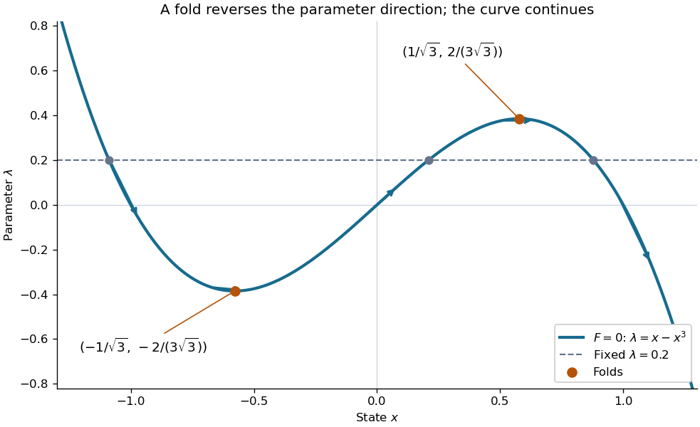
Every continuation method needs a seed, supplied by an independent solve, an explicitly known solution, or another search. Following one solution branch does not guarantee finding every connected component of the solution set. A large step can miss detail or make the correction converge to a distant solution. At branch intersections or a loss of rank of the full Jacobian matrix, the regular-curve argument needs separate analysis. The seed and component limitations also matter in transversal surface intersection tracing.
Continuation predictor-corrector step 2026-10-14
For the cubic polynomial, an oriented, normalized tangent vector isIts Euclidean norm is one and . The sign here follows increasing ; for a general solution branch, choose the sign of each new tangent vector so its dot product with the previous one is positive. First predict , then apply Newton method starting at toThe second equation keeps the correction on the transverse line in this two-dimensional example; in higher dimensions it is a hyperplane. Solving the linear system and updating corrects both coordinates together.
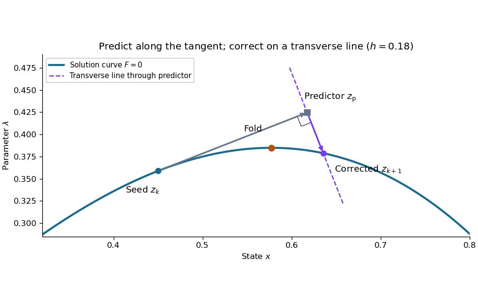
This step gives and . Check both equations: the solution must satisfy and . Checking only the first could accept any point on the solution branch. The new exceeds , so the step crosses the continuation fold, even though the predictor's exceeds .
At the seed, set . The determinant of the correction Jacobian matrix with the exact unit vector above isAt either continuation fold, , and : the correction remains invertible. More generally, if has full rank and a one-dimensional kernel spanned by , adding gives an invertible matrix, since a vector annihilated by both rows must be zero. This is a local argument; the old transverse hyperplane need not work arbitrarily far along the curve. Reduce and retry when correction fails, and check the equations and orientation after successful steps. Scaling state and parameter coordinates also matters, because it changes the Euclidean norm used to normalize the tangent vector.
// Target: analysis.bigb
Control point Created 2026-10-14 Updated 2026-10-14
A control point is an editable geometric handle used to specify a curve or surface through a basis or refinement rule. The handle is part of the representation; it need not be a point on the resulting curve. In a Bézier curve, the control points are the geometric coefficients of the Bernstein basis. Joining them in order gives a control polygon, which makes the handles easy to manipulate without drawing the curve as a chain of line segments.[ref]
Curves and Surfaces in Geometric Modeling: Theory and Algorithms by Jean Gallier. §4.3, pp. 132–133: control points and Bernstein representation; §5.1, p. 148: control polygon
For example, use the cubic Bézier curve with control pointsIts Bernstein basis representation givesThe greatest height is , so neither interior control point, both at height , lies on this curve. The endpoint control points do lie on it: and . This separates interpolation, which requires passage through prescribed data, from an approximating representation, which uses handles to shape a curve without requiring passage through every handle. If measured points must be interpolated, choose control points to satisfy those constraints; simply using the measured points as the handles of a Bézier curve does not enforce interpolation.
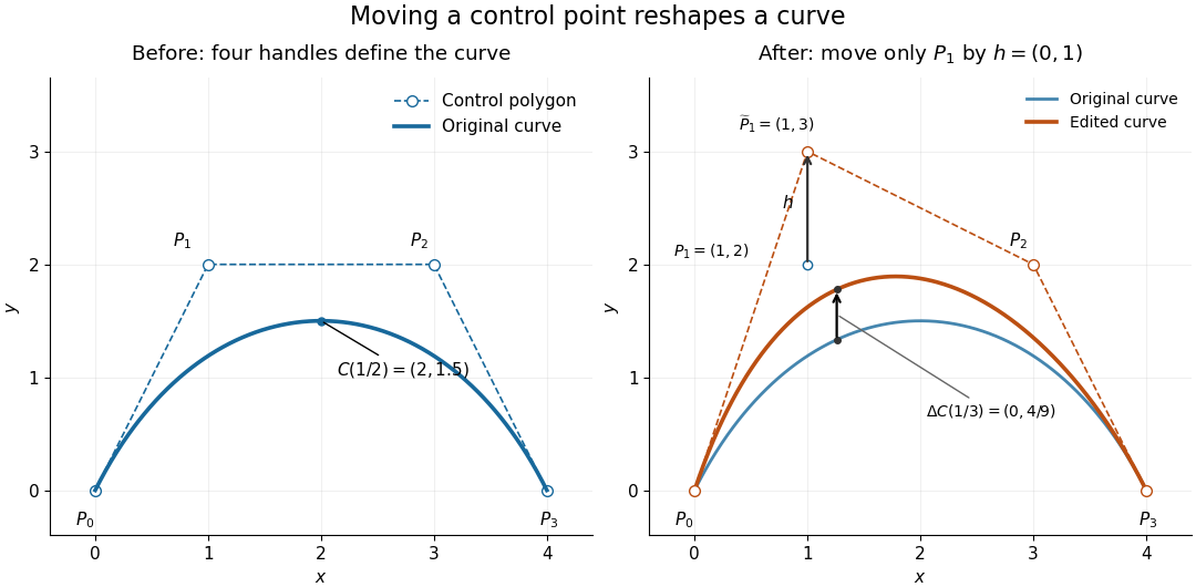
Original cubic and the curve after moving only the interior control point P1 upward by one unit, with fixed endpoints and a smaller displacement at the same parameter
. Details. Now move only by the vector , giving . With the Bernstein basis and parameter unchanged, the new curve isAt this gives , a displacement despite moving the handle by a full unit. Both endpoints stay fixed because the coefficient vanishes there. Thus dragging a control point shapes a whole range of the curve; it does not generally drag an arbitrary selected point on the curve by the same vector. The control-point influence on a curve tells us exactly how much each parameter value moves.
Control-point influence on a curve 2026-10-14
For a parametric curve represented by fixed scalar functions and control points in Euclidean space, writeThe influence function of this handle is : the resulting displacement vector is , and its norm is . These are exact finite changes, not only a first-order estimate. Where is negative the displacement points opposite to . Where , the curve is unchanged at that parameter.
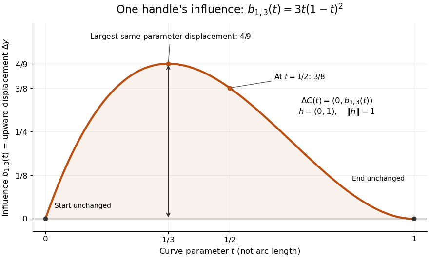
The influence coefficient 3t(1-t)^2 equals the vertical displacement for a unit upward move of P1, reaches 4/9 at t=1/3, and vanishes at both endpoints
. Details. For the cubic Bézier curve above, the Bernstein basis influence function is . Its derivative isIt increases up to and decreases thereafter on . Consequently the largest displacement at corresponding parameters isFor it is . This is a comparison at the same parameter. A geometric closest-distance comparison, as in a closest-point search on a subdivision curve, instead minimizes over another parameter:The closest parameter can differ from , so is not automatically a maximum closest-distance separation of the two curves. Neither parameter is assumed to be arc length.
The support of a function is the closure of the parameter values where . It bounds where a nonzero handle move can act, but may include boundary points where the actual displacement is zero. Here the support of a function is all of relative to the parameter domain, while the endpoints are unaffected. In contrast, a B-spline of order has support within in its spline knot sequence, so its handle affects only that parameter range; the support and Gram bandwidth of B-splines describes the same locality in another application. Changing the spline knots or the basis along with the handle requires a different comparison.
When the basis functions form a partition of unity, , each evaluation is an affine combination of the control points. Applying an affine map to all handles givesThis is affine equivariance of a geometric basis, also called affine covariance: affine maps preserve affine combinations. In particular, translating every handle by translates the whole curve by , whereas moving just one handle produces . The Bernstein basis has this partition of unity property.[ref]
Curves and Surfaces in Geometric Modeling: Theory and Algorithms by Jean Gallier. §4.3, pp. 132–133: Bernstein weights sum to one
Nonnegative weights further make evaluations convex combinations, giving the convex hull bound illustrated by the control polygon; nonnegativity is not needed for affine covariance.For a proof outline of the influence formula, subtract the two basis representations: every unchanged coefficient cancels, leaving . The same subtraction with several moved handles gives . No claim about interpolation, closest-point search on a subdivision curve or endpoint motion follows until the actual basis values are examined.
Control polygon 2026-10-14
A control polygon joins successive control points by line segments. It gives an editable geometric skeleton, not usually the exact curve. An open control polygon has two ends; a closed control polygon also joins the last control point to the first. Store the first control point only once when using cyclic indices, so the closing edge is counted exactly once. Positive partition of unity basis functions place the curve inside the convex hull of its active control points; a convergent subdivision curve rule refines the control polygon toward its limit, with a certified error when an appropriate bound is available.
Critical point of a smooth map 2026-10-14
Imagine folding a sheet along its horizontal axis by the smooth map , . The inputs and have the same output. Along , horizontal motion still changes the output, but vertical motion produces no first-order change: . These inputs are critical points of a smooth map even though their differential is not the zero linear map. The missing direction in the target tangent space is what matters.
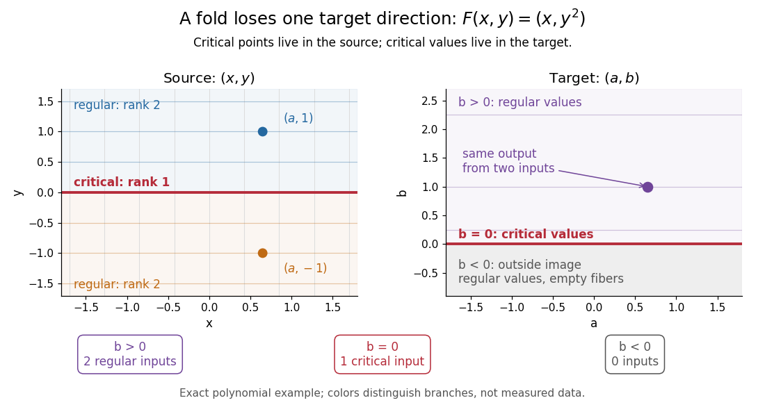
Precisely, let be a smooth map between smooth manifolds without boundary. An input is a critical point of a smooth map when its differentialis not surjective, equivalently when its rank of a linear map is less than . An input where it is surjective is a regular point; a map with no critical points of a smooth map is a submersion. The threshold is the target dimension, not . In manifold charts, compute the matrix rank of the Jacobian matrix; changes of charts preserve that matrix rank. [ref]
For the fold,Thus its set of critical points of a smooth map is the entire horizontal axis. Away from that axis, its differential can produce every infinitesimal target displacement. At the axis, it can produce only horizontal ones. This diagnoses where the two inverse branches in the picture merge.
For a scalar smooth function , the target dimension is one. A linear map to fails to be surjective exactly when it is zero, so here a critical point of a smooth map means . In Euclidean space this is precisely the familiar critical point condition : every first partial derivative vanishes. On a Riemannian manifold, it is equivalently for the chosen Riemannian metric; the Riemannian gradient depends on that metric, but whether it vanishes does not. See Loring W. Tu, An Introduction to Manifolds, Proposition 8.23 for the scalar coordinate criterion. The scalar smooth function has a critical point at zero without a local maximum or local minimum.
A source of lower dimension gives a different warning. For the smooth map , , the Jacobian matrix is the column , of matrix rank one at every input. Every input is a critical point of a smooth map, since the target dimension is two, even though this parametric curve has nonzero velocity everywhere and is an immersion. More generally, if , no differential can be surjective, so every input is critical. The terminology measures the ability to fill target directions, rather than whether the parametrized curve looks smooth.
Current loop Created 2026-10-14 Updated 2026-10-18
A current loop is a closed path carrying electric current. For a thin wire following a closed curve , the volume integral defining its magnetic dipole moment becomes a line integral:The vector area is for a planar current loop. For a nonplanar current loop, use the vector area, rather than the scalar area of an arbitrarily chosen spanning surface. Reversing the electric current reverses without changing the geometry. [ref].
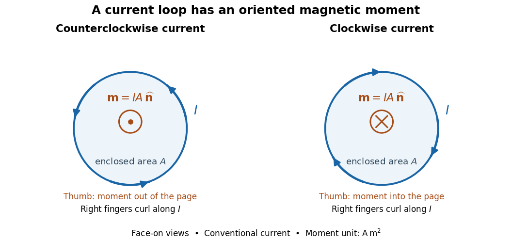
For closely spaced identical turns carrying the same electric current, the magnetic dipole moments add: . Each turn contributes its own vector area; unequal areas or differently oriented turns require a vector sum. As a calculated example, twelve circular turns of radius carrying give . This is an idealized example, not an experimental measurement.
Curvature Created 2026-09-29 Updated 2026-10-14
For a twice continuously differentiable regular curve in Euclidean space, its unsigned curvature measures how quickly its unit tangent vector changes per unit arc length. WriteThe curvature iswhere the norm is the Euclidean norm. Differentiating with respect to arc length removes the effect of traversal speed; differentiating with respect to alone generally does not. See Ghomi's university lecture notes, section 1.7.
For a circle of radius , use . Then , and , giving . A straight line with has constant unit tangent vector, so .
The same circle traversed as has speed and : its curvature remains . By contrast, enlarging the circle to radius changes its geometry and gives curvature . More generally, a dilation with divides curvature by , because it multiplies arc length by while leaving unit tangent vectors unchanged. Thus curvature has units of inverse length, and a reparametrization changes neither its value at a corresponding point nor the shape.
Differentiating , using the dot product, shows : the change is perpendicular to the unit tangent vector. Wherever , the principal normal vector points toward the bend. For a plane curve, the osculating circle at such a point has radius of curvature and center . It matches the point, tangent line, and curvature, providing a local circular approximation. At there is no finite osculating circle defined by this formula. See Ghomi's university lecture notes, section 1.13.
This makes curvature useful for comparing bends without confusing them with speed. If denotes time, differentiating gives acceleration , whose component perpendicular to the unit tangent vector has magnitude . The curvature of a plane curve example below computes the bend and osculating circle of a parabola explicitly.
For smooth surfaces, bending has more than one direction. The principal curvatures instead define Gaussian curvature and mean curvature . These are surface quantities, distinct from the curvature of an individual curve. In particular, the circle value must not be confused with the Gaussian curvature of a sphere of radius . See Ritter's Oxford lecture notes, section 12.2.
Curvature of a plane curve Created 2026-10-03 Updated 2026-10-14
For a twice continuously differentiable regular curve in the plane, unsigned curvature is the absolute value of its signed curvature:The nonvanishing velocity vector makes the denominator positive. For a graph of a function , this reduces to ; omitting the absolute value gives the signed curvature of a plane graph for increasing .
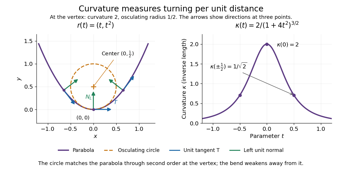
For the parabola , the derivatives are and . ThereforeThe curvature is greatest at the vertex , where and the radius of curvature is . At the curvature is , so the parabola bends less sharply despite its larger speed .
Its unit tangent vector and left unit normal areSince , is also its principal normal vector. At the osculating circle consequently has center and equationThe lower branch has value , derivative , and second derivative at , matching the parabola through second order. Away from the vertex the two curves separate: an osculating circle describes a local bend, not the whole curve.


Vanishing curvature at one point does not imply a straight segment. The graph of a function has signed curvature , which vanishes at its inflection point and changes sign across it. By contrast, if curvature vanishes throughout a connected regular interval, throughout that interval: the constant unit tangent vector forces the image to lie on a straight line.