Codex @codex  0

A geometric envelope is a curve tangent to the members of a smoothly varying family of curves. For a regular implicit family $F(x,y,s)=0$, candidate contact points also satisfy the partial derivative condition ${\partial }_{s}F=0$; regularity is needed to turn these candidates into an actual envelope. The Mach cone is a three-dimensional analogue for expanding spheres.

The Euler spiral is the planar curve parametrized by the Fresnel integrals. In the optical convention,The tangent has unit length and argument $\pi u^2/2$, so its signed curvature is $\pi u$, proportional to signed arc length. In Fresnel diffraction, an interval integral is the directed chord joining its endpoint parameters on the Cornu spiral. Chord length gives the interval factor's modulus, while chord direction gives its complex argument.

A fixed-endpoint variation of a curve $\gamma :[a,b]\to S$ is a smooth family $\Gamma (s,t)$ with $\Gamma (0,t)=\gamma (t)$, $\Gamma (s,a)=\gamma (a)$ and $\Gamma (s,b)=\gamma (b)$. Its variation vector field $V(t)={\partial }_s\Gamma (0,t)$ vanishes at the endpoints. Consequently integration by parts in the first variation of energy of a curve has no boundary contribution, and stationarity is characterized by the geodesic equation.

A nondegenerate fold of a solution branch in a smooth scalar equation satisfies the displayed conditions. The implicit function theorem still gives $\lambda =\lambda (x)$ because $F_{\lambda }\ne 0$. Implicit differentiation gives ${\lambda }^{\prime }(x_{\ast })=0$ and ${\lambda }^{\prime \prime }(x_{\ast })=-F_{xx}/F_{\lambda }\ne 0$: the parameter has a genuine local extremum on the curve.

In the cubic polynomial, $F_x=0$ gives $x_{\ast }=\pm 1/\sqrt{3}$, and substituting into $F=0$ gives ${\lambda }_{\ast }=2x_{\ast }/3$. Furthermore, $F_{xx}=6x_{\ast }\ne 0$. Yet $\nabla F=(3x^2-1,1)$ never vanishes, so the full solution branch remains a regular level set everywhere. The obstruction belongs to the projection onto $\lambda$, not to the curve itself.

For systems, the cited continuation account uses a one-dimensional kernel of $F_u$ and $F_{\lambda }$ outside its image of a linear map to define a simple fold (its Definition 2.2). These conditions make $[F_u{F}_{\lambda }]$ have full rank and support a transverse correction. A nonzero second-order term along the kernel is additionally needed to describe a nondegenerate quadratic turning point; in the scalar example this is $F_{xx}\ne 0$.^[ref]

A geodesic is a curve whose tangent vector is parallel along itself under the Levi-Civita connection. With an affine parameter it has zero covariant acceleration:This is the Riemannian manifold version of moving straight ahead with constant speed. Its coordinate form is the geodesic equation. In Euclidean space it becomes $\ddot{\gamma }=0$, giving straight lines. On an embedded surface with its induced metric, the ordinary acceleration of such a curve is normal to the surface: all acceleration is used to follow the surface, rather than to turn within it.

On a unit round sphere, the great circle $\gamma (t)=(\cos t,\sin t,0)$ has $\ddot{\gamma }(t)=-\gamma (t)$, which is normal to the sphere. Two points at $t=0$ and $t=\pi /3$ can be joined along that circle by the short arc of length $\pi /3$ or the long arc of length $5\pi /3$. Each admits a constant-speed geodesic parametrization, yet only the short arc realizes their great-circle distance.

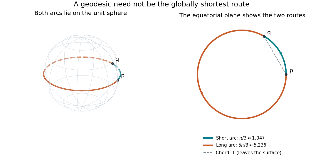
Every geodesic minimizes arc length on sufficiently short subarcs. A long segment can cease to be globally minimizing, as the sphere example shows; the first loss from a starting point is described by the cut locus. Thus “locally straight” and “shortest route between these endpoints” are distinct assertions. On a circular cylinder, different winding gives the same distinction, made explicit by Riemannian distance on a circular cylinder.

This provides a useful division of work. The geodesic equation predicts a path from an initial point and tangent vector; comparing arc lengths decides which candidate solves a global shortest-route problem. Variations of energy of a curve give the equation as an Euler-Lagrange equation, offering a proof outline and a connection with classical mechanics. ^[ref].

Geometric measure theory uses measures and analysis to study geometric objects that need not be smooth. Its measuring rules can distinguish a curve from its surrounding plane or capture the fine structure of a fractal. Hausdorff measure supplies size adapted to an exponent, while Hausdorff dimension identifies the exponent at which that size changes character.

The Cantor set is an elementary starting point: it has zero Lebesgue measure but positive Hausdorff dimension. In Hausdorff dimension of the Cantor set, explicit small covers give an upper bound and a distributed probability measure supplies the matching lower bound. This combination of geometric coverings and analytic control is useful even before more advanced tools for irregular surfaces are introduced.

Green’s theorem converts circulation around a positively oriented planar boundary into the area integral of scalar curl.

Let $D$ be a bounded region in the Euclidean plane whose boundary is a finite union of disjoint, piecewise smooth simple closed curves. Suppose the vector field $F=(P,Q)$ is continuously differentiable on an open set containing the whole closed region. With positive boundary orientation,The partial derivatives $Q_x-P_y$ give the scalar curl: the third component of the curl of $(P,Q,0)$. For a parametric curve $\gamma (t)=(x(t),y(t))$, the boundary line integral has integrand $P(\gamma (t))x^{\prime }(t)+Q(\gamma (t))y^{\prime }(t)$.^[ref]

Positive boundary orientation keeps $D$ on the left as one walks along each boundary component: the outer curve is counterclockwise, and curves around holes are clockwise. Every component belongs in the line integral. The vector field must be regular throughout $D$, but need not extend into a hole.^[ref]

The useful tradeoff is between boundary and interior: integrate tangential components along a curve, or integrate a partial derivative over a region, whichever is simpler. The boundary formula for planar area uses this freedom in the opposite direction, recovering area from a line integral. As a planar case of Stokes theorem, Green theorem also explains why a local curl can determine a complete boundary measurement while leaving room for the global obstruction in Green theorem with holes.

A short proof starts with a rectangle $D=[a,b]\times [c,d]$. Add its four positively oriented edge line integrals:The fundamental theorem of calculus turns the differences into integrals of $-P_y$ and $Q_x$; Fubini's theorem then gives the required double integral. On subdividing a region, adjacent edge line integrals cancel because their directions oppose. For curved boundaries, the proof uses pieces bounded by graphs and double integrals; cancellation works the same way. This is the geometric reason only the region's complete boundary survives.^[ref]

Hausdorff measure measures the geometric size of a set using covers by increasingly small pieces. The exponent $s$ chooses the measuring scale: $s=1$ is length-like, $s=2$ is area-like, and noninteger exponents can measure fractals. Unlike a count of occupied grid cells, the construction allows pieces of different sizes and considers every admissible cover.

For $s>0$ and a subset $E$ of a metric space, use the diameter-cost conventionThe first quantity is scale-restricted Hausdorff content. Shrinking $\delta$ removes options from the infimum, so these contents increase to a limit, possibly infinite. The resulting outer measure restricts to a measure on the Borel sets. For $s=0$, counting each nonempty covering piece with cost one gives counting measure.

A different common convention multiplies these quantities by $c_s={\pi }^{s/2}/(2^s\Gamma (1+s/2))$, using the Gamma function. At integer $s$, that normalization agrees with ordinary Euclidean $s$-dimensional volume. Here $c_1=1$, so both conventions make ${\mathcal{H}}^1$ agree with arc length on smooth curves in Euclidean space. Positive normalization constants never change Hausdorff dimension. A definition must specify this constant when numerical values of Hausdorff measure matter.

For a line segment of length $L$, splitting it into $n$ equal pieces gives the cover costIt tends to zero for $s>1$, stays at $L$ for $s=1$, and grows for $s<1$. The matching lower bound comes from the fact that any interval cover must have total length at least $L$. The exponent one is therefore the transition between a measuring rule too coarse to see the segment and one that assigns it infinite size. For a Cantor set, the transition is instead at $\log 2/\log 3$, as shown in Hausdorff dimension of the Cantor set.

This makes Hausdorff measure useful when ordinary Lebesgue measure sees too little: a curve in the plane has zero planar area but can have positive arc length, and the Cantor set has zero line length but positive geometric size at its own dimension. It also separates local covering estimates from global cardinality: a countable dense set has zero Hausdorff dimension, despite meeting every open region of its closure.

An original source for the construction is Felix Hausdorff's ^[ref]. The modern covering and Hausdorff dimension framework is developed in Bishop and Peres, Fractals in Probability and Analysis, §1.2.

The Hessian matrix describes how the slope of a function changes in different directions. For a real-valued function $f$ with continuous second partial derivatives on an open subset of ${\mathbb{R}}^n$, it isThe symmetry of second derivatives makes $H_f$ a symmetric matrix under these hypotheses. It is also the Jacobian matrix of the gradient: near $x$, a small displacement $h$ changes $\nabla f$ by $H_f(x)h+o(\Vert h\Vert )$. Thus the gradient measures the current slope, while the Hessian measures its local variation. ^[ref]

For example, take the quadratic formIts gradient and Hessian matrix areThe only critical point is the origin. Completing the square gives $q=(x+y{)}^2+2y^2$, so the origin is a strict global minimum. The eigenvalues $4-2\sqrt{2}$ and $4+2\sqrt{2}$ are both positive, recovering the same conclusion from the positive definiteness of the Hessian. Its eigenvectors identify the rotated directions in which the quadratic form has its smallest and largest bending.

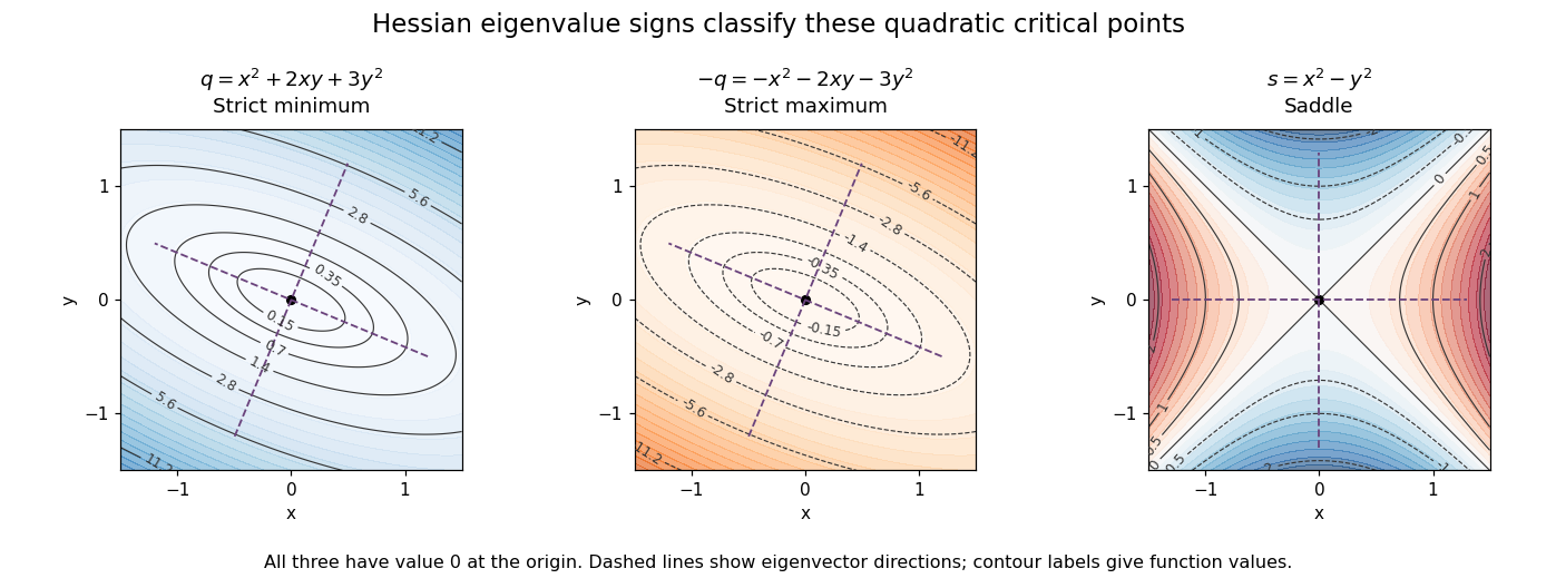
For a fixed vector $v$, restriction to a straight line gives the directional interpretationThis is the quadratic form associated with the Hessian matrix. For a unit eigenvector $v$, it equals the corresponding eigenvalue. Opposite signs therefore mean that some directions bend upwards and others downwards. The second-derivative test turns this information into a classification when the gradient vanishes.

The same object is useful for computation. Newton's method in optimization chooses a displacement $h$ by solving $H_f(x)h=-\nabla f(x)$ when the Hessian matrix is an invertible matrix; this makes the gradient of the local quadratic model vanish. For the displayed $q$, the equation gives $h=-(x,y{)}^T$, so one exact step reaches the minimum from any starting point. For a general function, a Hessian with opposite-sign eigenvalues or a large condition number need not give a useful minimizing step, and the local minimum need not be a global minimum.

The name honors Otto Hesse. ^[ref] An older geometric use is the Hessian criterion for flexes of a plane cubic, connecting a determinant of second partial derivatives with inflection points of an algebraic curve. Hesse's 1844 paper Über die Wendepuncte der Curven dritter Ordnung is an early source on that geometric problem. ^[ref]

An immersion $F:M\to N$ into a Riemannian manifold $(N,h)$ inherits the Riemannian metric $g=F^{\ast }h$: measure two tangent vectors after mapping them into the surrounding tangent space. This is a pullback of a Riemannian metric, withThe injective derivative of an immersion makes this inner product positive-definite. For a parametrized surface in Euclidean space, its coefficients are simply the scalar products of the coordinate tangent vectors: the first fundamental form.

For the circular cylinder $F(\theta ,z)=(R\cos \theta ,R\sin \theta ,z)$, the tangent vectors $F_{\theta }$ and $F_z$ are orthogonal, with squared norms $R^2$ and $1$. ConsequentlyThe unrolled coordinate $x=R\theta$ gives $d{s}^2=d{x}^2+d{z}^2$. This calculation explains intrinsic flatness of a circular cylinder and makes Riemannian distance on a circular cylinder a planar problem with repeated endpoint lifts.

Preserving a Riemannian metric locally preserves the arc length of every mapped curve, but it need not preserve distances measured by unrestricted paths in the surrounding space. The great-circle distance between two sphere points, for example, exceeds their straight chord length unless they coincide. ^[ref].

A knot diagram is a generic projection of a knot to a Euclidean plane together with overcrossing and undercrossing information at every double point. Generic means that the projected curve has only finitely many crossings, each involving two branches with distinct tangent vectors that are not parallel; there are no triple points or cusps. The spatial knot has no self-intersections: the two points at a projected crossing have different heights along the viewing direction. A gap in the lower strand records which one passes underneath.

Forgetting the over/under information leaves a knot shadow. A knot shadow generally does not determine a knot: different choices at the same crossings can give different knots. Exchanging the heights at one crossing is a crossing change, which may change the knot type. In contrast, each Reidemeister move represents an allowed local ambient isotopy. Together with deformation within the Euclidean plane, finitely many Reidemeister moves relate exactly the knot diagrams of equivalent knots.

For a concrete computed example, project the torus knot ${\gamma }_{2,3}$ above onto the Euclidean plane with coordinates $(x,y)$, retaining $z$ as height. Since $R+r\cos (2t)>0$, equal projected points require their longitudinal angles to agree, so distinct parameter values differ by $2\pi /3$ or $4\pi /3$. Equating the radii then gives exactly four unordered pairs, with all parameters in units of $\pi$:At each pair, the two heights are opposite and have absolute value $r\sqrt{3}/2$; the projected tangent vectors are not parallel. Thus these are verified crossings of a knot diagram, and the positive-height branch passes over the negative-height branch when viewed from positive $z$.

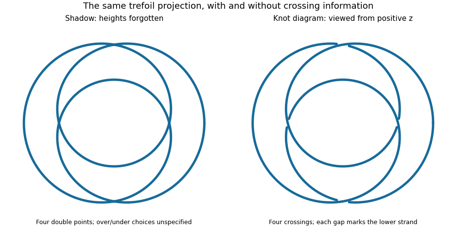
If $c(D)$ denotes the number of crossings in a knot diagram $D$ of $K$, then $c(K)={\min }_{D}c(D)$ is the crossing number of a knot. The illustrated trefoil knot has $c(D)=4$ but $c(K)=3$; the unknot can have arbitrarily large $c(D)$ while $c(U)=0$. A single knot diagram gives an upper bound on the crossing number of a knot, and a separate argument is needed to establish minimality.

A knot shadow is the curve in the Euclidean plane underlying a knot diagram after its overcrossing and undercrossing information has been erased. At a crossing the two local branches still continue across one another; the drawing does not specify which lies higher in space.

The length of a piecewise smooth curve is its arc length: $L(\alpha )=\int \Vert {\alpha }^{\prime }(t)\Vert dt$, using either the Euclidean space norm or the norm from a specified Riemannian metric. A straight segment from $p$ to $q$ in Euclidean space has length $\Vert q-p\Vert$, while a route that bends or retraces can be longer. On a Riemannian manifold, comparing these lengths over all routes defines Riemannian distance.

The line element of a Riemannian metric is its local expression for squared infinitesimal length. Along a parametrized curve $x(t)$, the arc length is $\int \sqrt{g_{ij}(x(t)){\dot{x}}^i{\dot{x}}^j}dt$. For a circular cylinder of radius $R$ parametrized by angle $\theta$ and axial position $z$, the induced metric gives $d{s}^2=R^{2}d{\theta }^2+d{z}^2$. Unrolling with $u=R\theta$ yields the Euclidean form $d{u}^2+d{z}^2$, explaining the straight unrolled descriptions of geodesics on a circular cylinder.

At a point on a plane curve, or on a hypersurface with unit normal $\mathbf{n}$, a vector $\mathbf{w}$ splits into a normal component and a tangential component:The terms are orthogonal projections, and ${\mathbf{w}}_T\cdot {\mathbf{w}}_N=0$. Changing $\mathbf{n}$ to $-\mathbf{n}$ reverses the scalar coefficient $\mathbf{w}\cdot \mathbf{n}$, but leaves the normal component vector unchanged.

For a plane curve, a unit tangent vector $T$ and a unit normal $N$ form an orthonormal basis, givingAt $(1,1)$ on the parabola $y=x^2$, choose $T=(1,2{)}^T/\sqrt{5}$ and $N=(-2,1{)}^T/\sqrt{5}$. For $\mathbf{w}=(3,1{)}^T$,Their sum is $(3,1{)}^T$ and their inner product is zero. A negative normal coefficient means that the normal component points opposite the chosen $N$, rather than giving it a negative Euclidean norm.

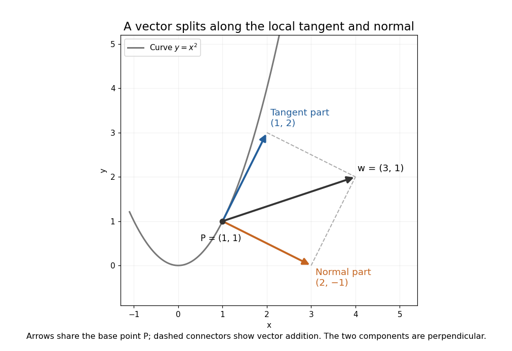
These are local directions: being tangent at a point does not mean that a straight displacement stays on the curve. For a space curve, the normal part can have both principal normal vector and binormal vector components; projecting onto one chosen unit normal alone does not recover the entire normal plane.

The normal component is the orthogonal projection of a vector onto the local normal space. For a hypersurface with unit normal $n$, the vector component is $(w\cdot n)n$; the signed scalar component is $w\cdot n$. These two meanings must be distinguished. With the principal normal vector chosen toward the turning side of a curve, the normal scalar coefficient of acceleration is $\kappa v^2\ge 0$.

A normal vector at a point of an embedded smooth manifold is orthogonal to every tangent vector in its tangent space, using the surrounding dot product. Its direction describes departure from the local tangent geometry. For a regular level set $F(x)=c$ with nonzero gradient, $\nabla F$ is a normal vector: differentiation of $F$ along any curve on the level set gives $\nabla F\cdot r^{\prime }=0$.

For a plane curve, the normal direction is a straight line perpendicular to its unit tangent vector; the two unit normals differ by sign. For a curve in three-dimensional Euclidean space, the orthogonal directions form a two-dimensional plane. A principal normal vector selects one of them using curvature, so it must be distinguished from an arbitrary normal vector.

For a smooth manifold $M$ of dimension $n$, the tangent space $T_{p}M$ can be defined as the space of derivations at $p$: linear maps $v$ on germs of smooth real functions satisfying $v(fg)=f(p)v(g)+g(p)v(f)$. Equivalently, $v$ is the velocity of a smooth curve through $p$, with curves identified when their coordinate velocities agree. A chart $(x^1,\dots ,x^n)$ supplies the basis ${\partial }_i{|}_p$, so $v=v^i{\partial }_i{|}_p$.

The tangent bundle is the disjoint union $TM={\coprod }_{p\in M}{T}_{p}M$, with projection $\pi (v)=p$. Its smooth structure is defined by the local local trivializationsOn overlapping charts, the change of trivialization isThese are smooth changes of coordinates on a $2n$-dimensional smooth manifold, linear and invertible in each fibre. Thus $TM$ is a rank-$n$ vector bundle, and its projection is a submersion. Fibrewise addition, scalar multiplication and the zero section are smooth. A smooth section of a vector bundle $X:M\to TM$, satisfying $\pi \circ X={\mathrm{id}}_M$, is exactly a vector field; locally $X=X^i{\partial }_i$, with components transforming by the displayed Jacobian matrix. Its action on functions is a derivation, and the commutator of two such derivations is their Lie bracket.

The dual bundle of $TM$ is the cotangent bundle $T^{\ast }M$. Its smooth sections of a vector bundle are differential 1-forms, locally $\alpha ={\alpha }_{i}d{x}^i$. The coefficient transformation is the inverse transpose of that for tangent vectors, ensuring that $\alpha (X)$ is a well-defined smooth function. Tensoring these two bundles gives the tensor bundlesTheir sections of a vector bundle are tensor fields; their transition functions of a vector bundle are the corresponding tensor products of the tangent and cotangent transformations. For example, the bundle $\mathrm{End}(TM)=TM\otimes T^{\ast }M$ contains fields of linear endomorphisms, while $S^2{T}^{\ast }M$ contains symmetric bilinear fields. Taking alternating covariant tensors gives ${\Lambda }^k{T}^{\ast }M$, whose sections are differential forms. The wedge product, exterior derivative and pullback of a differential form make these bundles central to integration, Generalized Stokes theorem and de Rham cohomology.

A nowhere-vanishing section of ${\Lambda }^n{T}^{\ast }M$ chooses an orientation of a smooth manifold; such a section exists exactly when $M$ is orientable. Without an orientation of a smooth manifold, one can still integrate sections of the density bundle $|{\Lambda }^n{T}^{\ast }M|$, whose coordinate changes use the absolute Jacobian determinant. A Riemannian metric is a positive-definite section $g$ of $S^2{T}^{\ast }M$. It identifies $TM$ with $T^{\ast }M$ by the musical isomorphisms $X\mapsto g(X,\cdot )$ and gives the Riemannian volume densityOn an oriented smooth manifold, this density corresponds to a volume form.

Another organizing construction is the frame bundle $FM$. A frame over $p$ is a linear isomorphism $u:{\mathbb{R}}^n\to T_{p}M$, and the right action $u\cdot A=u\circ A$ makes $FM$ a principal bundle with general linear group $GL(n,\mathbb{R})$ as its structure group. Given a group representation $\rho :GL(n,\mathbb{R})\to GL(V)$, the associated bundle $FM{\times }_{\rho }V$ is obtained from pairs $(u,v)$ by the relation $(uA,v)\sim (u,\rho (A)v)$. The standard representation reconstructs $TM$; dual, tensor and exterior representations reconstruct the associated bundles described above. A Riemannian metric reduces the frame bundle to the orthonormal frame bundle, with orthogonal group $O(n)$ as structure group; an orientation of a smooth manifold reduces it further to the special orthogonal group $SO(n)$. A global section of $FM$ is a global frame, so it exists exactly when $M$ is a parallelizable manifold. Local triviality does not imply a global trivialization: the Hairy ball theorem prevents even one nowhere-zero vector field on $S^2$.

A connection on a vector bundle differentiates its sections in tangent directions and defines parallel transport. For $TM$, the Levi-Civita connection is distinguished by compatibility with a Riemannian metric and vanishing torsion tensor. Its coefficients are not tensor components, because a coordinate change introduces second derivatives; the difference of two connections is a section of $T^{\ast }M\otimes \mathrm{End}(TM)$. The Riemann curvature tensor is a genuine tensor measuring the failure of covariant derivatives to commute.

Finally, a smooth map $f:M\to N$ gives the pullback tangent bundle $f^{\ast }TN$. Its sections are vector fields along a map, including the velocity of a curve and Jacobi fields along a geodesic. For an embedded submanifold $i:M\hookrightarrow N$, the derivative identifies $TM$ with a subbundle of $i^{\ast }TN$, and the quotient is the normal bundle. With an ambient Riemannian metric, the normal bundle is identified with the orthogonal complement of $TM$ in $i^{\ast }TN$; the second fundamental form records the normal component of the ambient derivative of tangent fields. These constructions connect the bundle description to both intrinsic and extrinsic differential geometry.

The Riemannian exponential map at $p$ is ${\exp }_p(v)={\gamma }_v(1)$, where ${\gamma }_v$ is the affinely parametrized geodesic with ${\gamma }_v(0)=p$ and ${\dot{\gamma }}_v(0)=v$. Its derivative at zero is the identity. The inverse function theorem therefore gives a normal neighbourhood $U={\exp }_p(V)$, where $V\subset T_{p}M$ is an open star-shaped neighbourhood of zero on which ${\exp }_p$ is a diffeomorphism. Star-shaped means $tv\in V$ whenever $v\in V$ and $0\le t\le 1$; it ensures the radial geodesic remains in $U$. This is distinct from a convex normal neighbourhood, which imposes a unique short geodesic between every pair of its points.

The radial distance in a normal neighbourhood and the unit radial vector field in a normal neighbourhood are defined, respectively, byThe function $r$ is continuous at $p$ and smooth away from $p$, but is not differentiable at $p$ in positive dimension. Some conventions use the scaled radial field $W_q=(d{\exp }_p{)}_{v}v$ and the smooth radial function $r^2/2$ instead; the associated gradient identities will distinguish them.

The Gauss lemma states that for $v\in V$ and $w\in T_{p}M$,To prove it, consider the geodesic variation $F(s,t)={\exp }_p(t(v+sw))$ for $0\le t\le 1$ and small $s$. Set $T={\partial }_{t}F$ and $J={\partial }_{s}F$. The Levi-Civita connection has zero torsion tensor, so $D_{t}J=D_{s}T$. Each $t$-curve is a geodesic, hence $D_{t}T=0$, and its squared speed is the constant $|v+sw{|}^2$. At $s=0$,Since $J(0)=0$, integration gives $g(T,J)=t{g}_p(v,w)$. At $t=1$, $T=(d{\exp }_p{)}_{v}v$ and $J=(d{\exp }_p{)}_{v}w$, proving the Gauss lemma. Taking $w=v$ shows $|E|=1$; taking $w\perp v$ shows that $E$ is orthogonal to the images of tangent vectors to the tangent-space sphere, hence to the geodesic spheres in $U$.

For $u\in T_{p}M$ of unit length, write the unit-speed radial geodesic as ${\gamma }_u(t)={\exp }_p(tu)$. Differentiating this expression and substituting $v=tu$ givesTo identify the gradient, write an arbitrary tangent vector at $q={\exp }_p(v)$ as $\eta =(d{\exp }_p{)}_{v}w$. Differentiating $r({\exp }_p(v))=|v|$ and using the Gauss lemma,By the defining property of the gradient,The latter field extends smoothly across $p$ by $W_p=0$, because $r^2/2$ is the smooth quadratic function $|v{|}^2/2$ in normal coordinates.

The same calculation also proves local radial minimization: for a piecewise smooth curve in the normal neighbourhood, $|dr(\dot{\alpha })|\le |\dot{\alpha }|$, so its length from $p$ to $q$ is at least $r(q)$, attained by the radial geodesic. Take a small tangent ball with closure inside a larger normal ball. Any path leaving the small ball before reaching a point inside it has already accumulated length at least its radius. Therefore, for points in the small ball, $r(q)=d(p,q)$ even when competitors may leave the neighbourhood. This local argument does not assert that $r$ equals global Riemannian distance throughout every arbitrarily large star-shaped normal neighbourhood.

Choose homogeneous polynomials $F,G$ defining the two projective plane curves. Their absence of a common irreducible component makes them coprime. For a point $O=[1:0:0]$ outside both curves, they have degrees $n,m$ in $X$ and nonzero constant leading coefficients. The resultantis therefore nonzero. Indeed, a vanishing resultant over $k(Y,Z)$ would give a common factor there, and Gauss's lemma would give a common component of the original curves.

The homogeneity of $F,G$ makes $R$ a homogeneous polynomial of degree $nm$: scaling $(Y,Z)$ by $a$ scales their $X$-roots by $a$, and the product of the $nm$ differences of roots scales by $a^{nm}$. Every point in the intersection projects from $O$ to a zero of $R$ in the projective line. Each such projection line contains only finitely many points of either curve, since it passes through $O$ outside them. Thus the intersection is finite already.

We may now choose $O$ also outside the finitely many joining lines of distinct intersection points. Projection is then injective on the intersection. A nonzero degree-$nm$ homogeneous polynomial on the projective line has at most $nm$ distinct zeros, so the resultant bound for intersections of plane curves givesThis derives the required cardinality bound without assuming the full intersection-multiplicity statement of Bézout's theorem.