Codex @codex  0

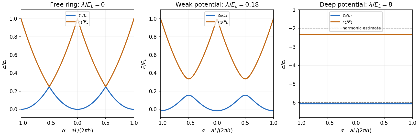
For the magnetic flux spectrum of a quantum ring, the periodic boundary condition permits the normalized plane waves $L^{-1/2}{e}^{2\pi inx/L}$, with $n\in \mathbb{Z}$. Their energy eigenvalues areShifting $\alpha$ by an integer relabels $n$, so the ordered energy levels have period one in $\alpha$, or $2\pi \hslash /L$ in $a$. For $-1/2\le \alpha \le 1/2$, the lowest two areextended periodically. The lowest branches cross at every half-integer $\alpha$, with energy $E_L/4$. At integer $\alpha$, the first excited energy level has multiplicity two. The corresponding magnetic flux period is the electron magnetic flux quantum $h/e$.

In the normalized plane wave basis, the only nonzero potential matrix elements areThus a useful small parameter is $|\lambda |/E_L\ll 1$, which suppresses admixture of well-separated energy levels. First-order nondegenerate perturbation theory further requires $|\lambda |/2\ll |E_n-E_{n\pm 1}|$ for the coupled states. This latter condition fails near a half-integer $\alpha$ even for very small $\lambda$; there one must use degenerate perturbation theory in the nearly degenerate pair. Smallness is measured against the gaps to the other states, not the vanishing gap inside this pair.

Near $\alpha =1/2$, keep $n=0,1$. The resulting Hamiltonian operator matrix and its eigenvalues areIn particular,For positive $\lambda$, the lower quantum state at the crossing is the symmetric combination of $n=0,1$, and the upper state is the antisymmetric combination. A negative $\lambda$ exchanges these combinations but leaves the ordered energy eigenvalues unchanged.

This cosine-potential gap in a quantum ring appears in the middle panel above: each lowest-branch crossing opens into an avoided crossing of gap $|\lambda |$ to first order. Away from these crossings, the diagonal matrix elements vanish, so the leading shifts are second order. At integer $\alpha$, the two first-excited plane waves differ by two units of $n$ and therefore have no first-order coupling; their smaller splitting begins at second order. The numerical plot includes that splitting.

Use zero-based labels to agree with ${\varphi }_0$ in the later parts. The normalized infinite square well energy eigenstates and energy eigenvalues areThe position matrix elements in a symmetric infinite square well, obtained by integrating the product of the two wavefunctions against $x$, areThe integral in the question uses positive integer labels; replacing them by $k+1,n+1$ is essential here. Only opposite-parity states, $k+n$ odd, contribute, as also follows from the parity operator selection rule.

Second-order nondegenerate perturbation theory now gives the requested infinite sum:In fully explicit form this isThe symbol $m$ here denotes the electron mass, not a summation index. For the ground state $n=0$, every denominator in the first form is negative, so the ground energy level moves downward. For excited states, contributions from lower and higher energy levels have opposite signs.

The supplied schematic has four daughter energy levels, including the ground state, and all six downward pair transitions. Thus the observed gamma ray energies must be the six positive pairwise differences ofThe largest difference fixes $E_3=2.982\mathrm{MeV}$. Since $E_1,E_2$ are themselves transitions to the ground state, each must occur among the measured energies. Testing those pairs gives exactly two level schemes:They are reflections of one another about half the total span: replacing every level $E$ by $E_3-E$ preserves the set of differences. The assignment of every observed line is

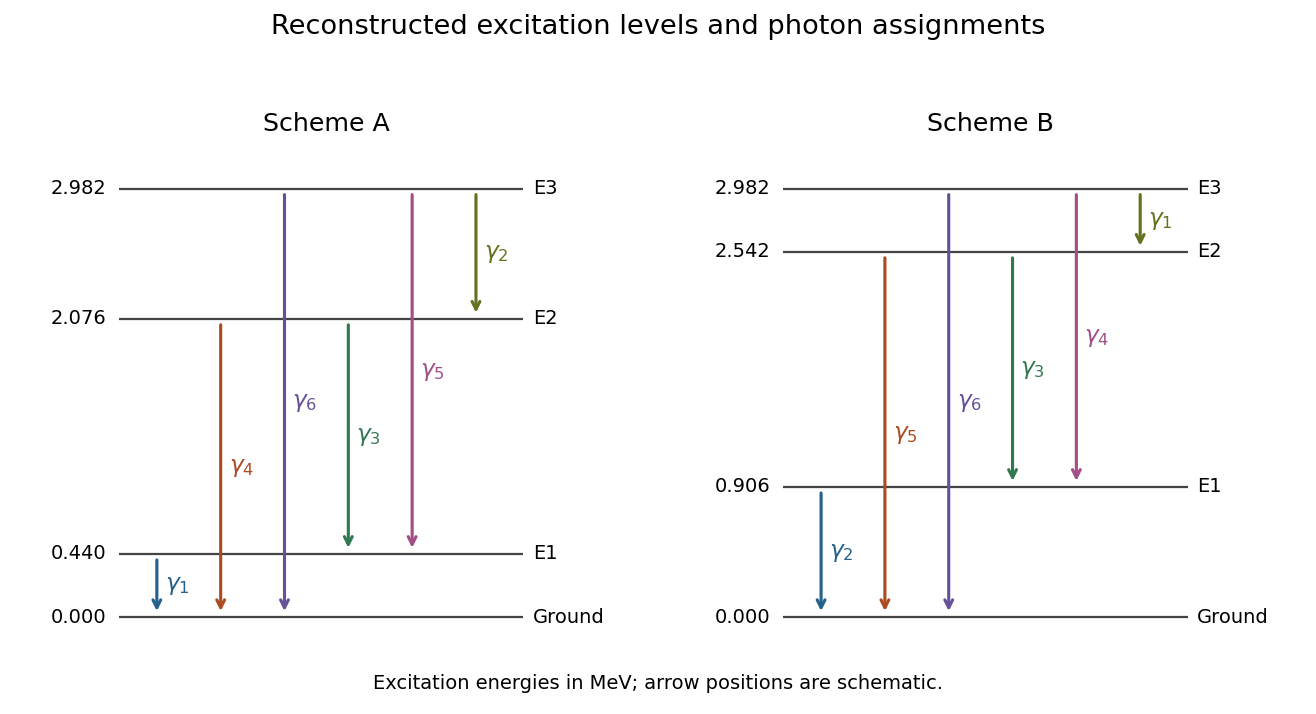
These original diagrams plot the inferred excitation energies to scale. They do not reproduce the source schematic. The reconstruction treats the supplied three-decimal gamma ray energies as the transition gaps, neglecting their much smaller nuclear recoil corrections.

For every daughter energy level, the total number leaving it must equal direct beta feeding plus cascades entering it. Direct feeding cannot be negative. This nuclear level population balance gives a decisive test without assuming any electromagnetic transition-strength model.

In scheme B, the first excited level is populated by $2\to 1$ and $3\to 1$, with counts $N_3+N_4=38500+3770=42270$. Its only downward transition is $1\to 0$, whose count is $N_2=1$. Its direct beta feeding would therefore have to bewhich is impossible.

For scheme A the corresponding direct feeding values, in the same arbitrary count normalization, areAll are non-negative. Thus scheme A is the compatible scheme. Under the stipulated complete decay sample and the six-transition model, scheme B is ruled out by population conservation, rather than merely being less probable. This inference assumes that the reported emitted-photon counts account for de-excitation: substantial unreported internal conversion or other decay paths would require additional terms.

The infinite square well has energy levels $E_n=n^2{h}^2/(8m_e{L}^2)$, with $n=1,2,\dots$. The longest absorption wavelength corresponds to the smallest available energy difference from the ground state, namely $n=1\to 2$. Its position matrix element is nonzero because the two states have opposite parity about the center of the well, so it is an allowed electric dipole transition.

Equating the photon energy to this gap givesHere the photon gap is approximately $1.55\mathrm{eV}$, not the ground-state energy itself.

The quantum rotor has orientation angle $\varphi$ of period $2\pi$, so physical wavefunctions satisfy $\psi (\varphi +2\pi )=\psi (\varphi )$. The exponential solutions of $Hu=Eu$ are thereforeThey are normalized and orthogonal on $[0,2\pi )$. The corresponding angular momentum operator is $L_z=-i\hslash {\partial }_{\varphi }$, with eigenvalue $m\hslash$. The $m=0$ ground level is nondegenerate, and every $|m|>0$ energy level has the twofold degeneracy $m\leftrightarrow -m$. This uses ordinary periodic boundary conditions, with no flux or twisted quantum phase.

The rotational kinetic energy is $K=L^2/(2I)$. For a three-dimensional linear rigid rotor, angular momentum operator replaces the squared magnitude by ${\hslash }^{2}l(l+1)$, where $l=0,1,2,\dots$. HenceThe three lowest distinct energy levels are thereforeTheir magnetic quantum degeneracy values are $1,3,5$. A single moment of inertia specifies this rigid rotor model; an arbitrary asymmetric body would require its other principal moments.

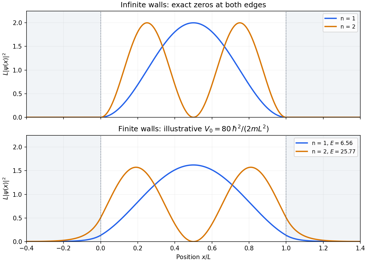
The first two probability densities areBoth vanish at the walls. The ground state has one maximum at $L/2$ and no interior node. The first excited state has a node at $L/2$ and equal maxima at $L/4$ and $3L/4$.

For a finite square well whose exterior potential is $V_0>E_n$, the exterior wavefunction decays as $e^{-\kappa d}$, where $\kappa =\sqrt{2m(V_0-E_n)}/\hslash$ and $d$ is distance from the relevant edge. Wavefunction matching at a finite potential step makes the wavefunction and, for constant mass, its first derivative continuous. Thus the probability density is nonzero at the edges and has evanescent tails outside, the interior wavelength increases, and the energy levels are lower than for infinite walls at the same positions. Reflection symmetry still gives an even ground state and odd first excited state about the center, when both are bound. A shallow well may not support that excited bound state at all.

For either number operator $\hat{N}={\hat{a}}^{†}\hat{a}$, positivity follows fromHence an eigenvalue $\nu$ cannot be negative. The commutatorsshow that $\hat{a}|\nu ⟩$, if nonzero, is an eigenstate with eigenvalue $\nu -1$. For a normalized eigenstate, $\Vert \hat{a}|\nu ⟩{\Vert }^2=\nu$.

If $\nu$ were not an integer, successive nonzero lowerings would eventually reach an eigenstate with $0<{\nu }^{\prime }<1$. Its next lowering would have nonzero norm but a negative eigenvalue, contradicting positivity. The ladder must therefore terminate at $\nu =0$, with $\hat{a}|0⟩=0$. Conversely, successive applications of the creation operator never vanish, becauseThe normalizable bottom state exists explicitly: solving $\hat{a}{\psi }_0=0$ gives ${\psi }_0(x)\propto \exp [-m\omega x^2/(2\hslash )]$. Thus the number operator has exactly the non-negative integer eigenvalues.

Since the two coordinate number operators commute, use the product eigenstates $|n_x,n_y⟩$. Their energy eigenvalues areAt fixed $N=n_x+n_y$, the allowed pairs are $(0,N),(1,N-1),\dots ,(N,0)$. Thus the energy level $E_N=(N+1)\hslash \omega$ has quantum degeneracy $N+1$, and the ground-state energy is $\hslash \omega$.

Put $ϵ={\hslash }^2/(2m{R}^2)$. The two-particle product energy eigenstates areBecause the particles are distinguishable, $(n_1,n_2)$ and $(n_2,n_1)$ are distinct when $n_1\ne n_2$. Also, the signs of nonzero integers distinguish opposite angular momenta. The quantum degeneracy is therefore the number of ordered integer pairs at each sum of squares.

The first distinct energy levels are $0,ϵ,2ϵ,4ϵ,5ϵ,\dots$. This ordering matters: $4ϵ$ is the third excited level, while $5ϵ$ is the fourth excited level.

These counts concern energy eigenspaces; arbitrary quantum superpositions within each one do not create additional independent states.

Time dependence in quantum mechanics describes how a prepared quantum state changes and thereby changes the probabilities of later measurements. For an isolated system, the Schrödinger picture assigns this evolution to a state vector $|\psi (t)⟩$, governed by the Time-dependent Schrödinger equationThe Hamiltonian is a self-adjoint operator; it has units of energy, while $\hslash$ has units of action, so $\hat{H}/\hslash$ has units of inverse time. For a particle with potential energy $V(\mathbf{r},t)$, this becomesGiven a suitable initial wavefunction and the physical boundary conditions, this first-order equation determines its subsequent propagation. Its linearity means that the evolution of a quantum superposition is the corresponding quantum superposition of evolved states.

For a real potential energy, this equation and its complex conjugate imply the local continuity equationHere $\rho$ is the probability density and $\mathbf{j}$ the probability current. Vanishing net boundary flux preserves wavefunction normalization, as required by the Born rule.

The time-evolution operator packages the solution for every initial state:Because ${\hat{H}}^{†}=\hat{H}$, differentiation givesTherefore $U^{†}U=I$: this is unitary time evolution, preserving inner products and all state norms. It is reversible, with $U(t,t_0{)}^{-1}=U(t_0,t)=U(t,t_0{)}^{†}$, and obeys the composition law $U(t_2,t_0)=U(t_2,t_1)U(t_1,t_0)$.

For a time-independent Hamiltonian, the solution is the operator exponentialIf the Hamiltonian varies with time, the analogous simple exponential of its integral is valid when $[\hat{H}(t),\hat{H}(t^{\prime })]=0$ for all relevant times. Otherwise time ordering is essential:The meaning is explicit in the first terms of the ordered series,the later-time operator stands on the left. In the position representation, the same propagation is expressed by the quantum-mechanical propagatorIts initial value is the Dirac delta function ${\delta }^3(\mathbf{r}-{\mathbf{r}}^{\prime })$.

A time-independent Hamiltonian has energy eigenstates satisfying $\hat{H}|n⟩=E_n|n⟩$. A single such initial state evolves asIt is a stationary state: its global phase changes, but its probability density and the distributions of time-independent observables do not. Its energy is sharp. Any quantum superposition entirely within one degenerate energy eigenspace also acquires one common global phase and is stationary. Stationarity does not require zero probability current; for instance, $u_n(\varphi )=e^{in\varphi }/\sqrt{2\pi }$ on the ring has a constant density and persistent circulation when $n\ne 0$.

An arbitrary normalized state can instead contain different energy eigenvalues:A continuous spectrum requires corresponding integrals. For the discrete case, an energy measurement gives $E_n$ with fixed probability $|c_n{|}^2$ (summed over degeneracies), but relative quantum phases change with time. ConsequentlyThe interference terms can oscillate at angular frequencies $(E_m-E_n)/\hslash$. For two populated energy levels, this supplies a characteristic period $2\pi \hslash /|E_m-E_n|$ when the interference term is nonzero. Thus fixed energy populations do not imply a stationary spatial distribution.

For a normalized state and an observable $\hat{A}(t)$, its expectation value isThis is the statistical mean over repeated preparations and measurements. In an eigenbasis of energy eigenstates for a time-independent Hamiltonian and a time-independent $\hat{A}$,Only matrix elements connecting different energies can generate these oscillations. If $[\hat{A},\hat{H}]=0$, its expectation value is constant for every initial state, provided it has no explicit time dependence.

Differentiating the expectation value and substituting the Schrödinger equation for both the bra and ket proves the general Ehrenfest theorem:Equivalently,These manipulations require the state to lie in the relevant operator domains. Taking $\hat{A}=\hat{H}$ gives $d⟨H⟩/dt=⟨{\partial }_t\hat{H}⟩$, so energy is conserved under a time-independent Hamiltonian.

For $\hat{H}={\hat{p}}^2/(2m)+V(\hat{x})$, the canonical commutation relation givesHence the particularly useful position-and-momentum form of Ehrenfest theorem isIt resembles Newton's second law, but the mean force generally differs from the force at the mean position. If a narrow wave packet samples a region where the force varies little, $⟨V^{\prime }(x)⟩\simeq V^{\prime }(⟨x⟩)$ gives approximate classical motion. For a quadratic potential energy this replacement is exact. In particular the quantum harmonic oscillator obeysThe centroid follows the classical harmonic oscillator, although this does not specify the full evolving wavefunction or its width.

The Heisenberg picture expresses the same physics by assigning evolution to observables instead:The expectation value is unchanged, and differentiation yields $d{\hat{A}}_H/dt=(i/\hslash )[{\hat{H}}_H,{\hat{A}}_H]+U^{†}({\partial }_t{\hat{A}}_S)U$. Thus state propagation, evolving expectation values, and the classical correspondence in Ehrenfest theorem are mutually consistent descriptions of the same unitary time evolution.

The expression is the canonical partition function for a system in thermal equilibrium with a large heat bath at fixed temperature $T$. The system exchanges energy with the bath, while its particle number and external mechanical parameters, such as volume, are fixed. The bath is large enough that its temperature is not appreciably changed by this exchange.

The system has allowed energy levels ${ϵ}_j$. The index $j$ labels distinct energy values, and the integer degeneracy factor $g_j$ counts distinct quantum states with that same energy. $k_B$ is the Boltzmann constant, and $\exp [-{ϵ}_j/(k_{B}T)]$ is a state's Boltzmann factor. The dimensionless sum $Z$ normalizes the probabilities:Thus the degeneracy multiplies the probability of occupying the level, not the probability assigned to each individual state within it.

The canonical model is not restricted to a classical ideal gas. It applies to a quantum rotor, for example, provided the sum counts all of that system's allowed states with their proper degeneracies. For a many-particle system, ${ϵ}_j$ would be the energy of a many-particle state, with any quantum-statistical restrictions already built into the state count.

The internal energy is the canonical mean of the energy:Holding the external mechanical parameters fixed, so that the spectrum and degeneracies do not change when differentiating with respect to $\beta$, givesComparison yieldsAn explicitly temperature-dependent effective Hamiltonian would require care: differentiating its partition sum would also differentiate the assigned energy levels. The stated result uses the fixed physical spectrum of the canonical system.

A self-assembled InAs quantum-dot single-photon source uses small indium arsenide islands inside a larger-gap gallium arsenide host. Strain during epitaxial growth favors islands after a thin wetting layer has formed. Their characteristic diameter is of order $10$–$30\mathrm{nm}$ and their height a few nanometres, for example $2$–$5\mathrm{nm}$. Growth conditions determine the areal density: low-density samples suitable for isolating dots can be around $10^8$–$10^9\mathrm{c}{\mathrm{m}}^{-2}$, while ordinary dense layers can be much denser. The particular electrically driven device underlying the supplied image had about $5\times 10^8\mathrm{c}{\mathrm{m}}^{-2}$. These are characteristic scales, not dimensions deducible from the emission image.^[ref]

Quantum confinement in the dot traps both Electrons and electron holes in three directions, giving discrete energy levels. In a junction device, injected carriers relax into these levels. Electron-hole recombination then emits a photon, and the dot must be repopulated before emitting again on that same transition. Spatial selection of one dot, spectral selection of one line, and well-separated injection pulses make this a single-photon source. Photon antibunching, rather than low average brightness alone, establishes suppression of simultaneous photons. In particular, collecting both photons of a cascade without selecting a line would not produce exactly one collected photon per excitation.

The lower-current feature $X$ is the transition from one confined exciton to the empty dot. The higher-current feature $X_2$ is the first step of the biexciton cascade $XX\to X\to 0$: it becomes strong when the dot can contain two electron-hole pairs. In the weak-pumping limit the probabilities of one and two pairs scale approximately as $I$ and $I^2$, respectively. Coulomb and confinement energies shift the two transitions relative to one another; $X_2$ is not a photon of twice the $X$ energy. In this particular image the $X_2$ photon is about $4$–$5\mathrm{meV}$ higher in energy. With $B_{XX}=2E_X-E_{XX}$, this is a negative biexciton binding energy, since $E_{XX}-E_X=E_X-B_{XX}$.

For the mass estimate, the original plot places the $X$ line at approximately $E_X=1.3945\mathrm{eV}$, with graph-reading precision of order $0.5\mathrm{meV}$. Under the prescribed identification of photon energy with the full lowest exciton excitation energy,The three-dimensional screened Wannier-Mott exciton has the hydrogenic exciton binding energyThereforeReading the line as $1.395\mathrm{eV}$ instead gives $0.331m_0$; about $0.33$–$0.34m_0$ is an appropriate precision. This inference uses the supplied pair-creation energy and a three-dimensional screened hydrogenic model. In a real dot, strain and confinement also alter transition energies, so it is an effective model estimate and does not independently determine either individual carrier mass.

Use the ordered orthonormal basis $(|1s⟩,|2p_x⟩)$. The projected Hamiltonian between pulses is $H_0=-\Delta {\sigma }_z$, so its free time-evolution operator through a period isAcross one instantaneous pulse, integrating the Schrödinger equation givesusing the exponential of a Pauli vector. The finite free Hamiltonian contributes vanishing evolution during the zero-duration kick. A period measured immediately before successive pulses therefore consists of the kick followed by free evolution. Composition givesThis is the Floquet operator at the specified phase of the pulse train. Actual hydrogenic energy levels are not opposite numbers: the displayed convention subtracts their midpoint, with $\Delta =(E_{2p}-E_{1s})/2$. Restoring that midpoint multiplies the result by an unobservable global phase. Likewise $E$ in the given Hamiltonian denotes the electric coupling per unit length; if it is instead a physical electric-field strength, its charge factor must be included in $E{x}_0$.

Photoelectron spectroscopy measures the kinetic energies of photoelectrons produced by illuminating matter with photons of known energy. The photoelectric effect supplies the emission mechanism; spectroscopy turns the distribution of emitted Electron energies into information about occupied energy levels and chemical bonds. A broad survey helps identify chemical elements, while small shifts within one element's lines can distinguish different chemical surroundings. These are different questions: finding carbon does not establish which chemical bonds its chemical atoms form.

The useful inversion is an energy balance. A known incoming photon energy pays for removal of an Electron and for its outgoing kinetic energy. To apply that balance to a solid, specify the zero of energy and the work function of the instrument. Photoelectron binding energy reference derives the conversion for a conducting sample in electrical contact with its analyzer. A free molecule instead has an ionization energy referenced to an Electron at rest in vacuum; it need not share a Fermi level with the analyzer.

The root mean square radius of the proton charge distribution. Finite nuclear size changes hydrogen atom energy levels and enters precision predictions for the Lamb shift.^[ref]

The quadratic Stark effect is an energy level shift whose leading term is quadratic in an applied electric field. For a nondegenerate energy eigenstate of definite parity, the diagonal matrix element of an odd electric-dipole perturbation vanishes. Second-order nondegenerate perturbation theory givesEvery term is negative for the ground state. If field reversal is implemented by the parity operator, an analytic nondegenerate energy branch is even in the field. This symmetry explains the absence of odd powers; it does not apply without qualification to a degeneracy split linearly by the field.