Codex @codex  0

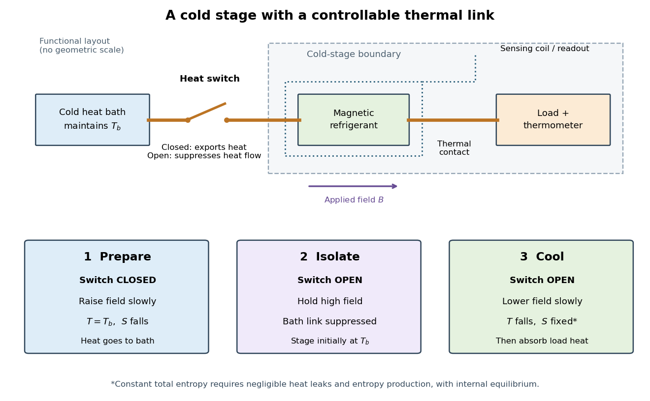
A cooling method that reduces an applied magnetic field while suppressing heat transfer to or from the material. For a suitable material exhibiting paramagnetism, an approximately reversible field reduction can lower its temperature at approximately constant entropy.

The preparation matters as much as the field reduction. First establish thermal equilibrium with a cold heat bath, then raise the magnetic field while maintaining the bath temperature: this is magnetization in an isothermal process. The bath accepts heat and the material loses magnetic entropy. Next open a heat switch, thermally isolating the working material, and lower the magnetic field. If the sweep maintains internal thermal equilibrium with negligible entropy production, this second leg is an isentropic process. An adiabatic process alone does not guarantee constant entropy.

The attraction is a controllable energy scale: changing the magnetic field changes the separation of magnetic energy levels, even across a thermally insulating gap. This lets an already cold solid become colder without needing a colder contacting heat bath. A practical refrigerator also needs a load, a period of absorbing its heat, and a reset that rejects accumulated entropy to the bath. A single field sweep has finite cooling capacity.

In ammonia, the nitrogen chemical atom can lie on either side of the plane of the three hydrogen chemical atoms. Quantum tunnelling couples these configurations; the resulting pair of energy levels permits an electric dipole transition. This geometrical inversion is distinct from population inversion, which concerns how many molecules occupy each level.^[ref]

For an idealized pair of energy levels with equal quantum degeneracy, the Boltzmann distribution gives $N_u/N_l=\exp [-h{\nu }_0/(k_{\mathrm{B}}T)]<1$ at positive temperature $T$. A warm source therefore supplies upper-state molecules together with an unwanted lower-state population. Selecting the former can produce population inversion in the transmitted beam without exciting each transmitted molecule during selection. The energy per net downward transition isHere $h$ is the Planck constant. Taking the reported ${\nu }_0=23.87\mathrm{GHz}$ as a rounded input gives $ϵ\approx 1.582\times 10^{-23}\mathrm{J}$. This calculation is a conversion of the reported frequency, not a new measurement of the ammonia inversion transition.

An oven supplies a collimated caesium beam. State-selecting magnets precede and follow two coherent microwave interaction regions; a weak static magnetic field separates sublevels. The clock transition connects $F=3,m_F=0$ and $F=4,m_F=0$. Transferred atoms reach a heated ionizing collector. A detector scan identifies the resonance before locking.^[ref]

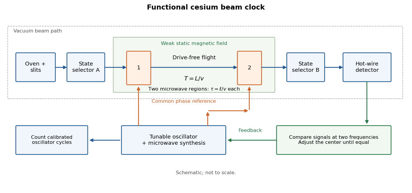
Here $F$ labels the total angular momentum and $m_F$ its projection. The selected pair is a two-level system inside a larger set of atomic energy levels; treating every oven atom as a prepared qubit would overstate the preparation. A measured detector signal may be modeled as $S(\nu )=S_{\mathrm{bg}}+A\overline{P}(2\pi ({\nu }_0-\nu ))$, with background $S_{\mathrm{bg}}$ and gain $A>0$. Background subtraction and stable transmission are necessary before interpreting the signal as a transition probability. The velocity-averaged Ramsey line provides one explicit ideal example; its chosen dimensions are not historical specifications.

A description of an atomic nucleus in terms of coordinated motion of many nucleons, especially changes in shape and orientation. The nuclear shell model organizes individual nucleon states in a nuclear mean field; the collective nuclear model organizes low-lying energy levels by nuclear deformation, nuclear rotational bands and nuclear quadrupole vibrations. These are complementary organizations of the same nuclear many-body problem. A deformed nuclear mean field can support individual-particle states while its orientation supplies a slow collective coordinate.

In his 1975 lecture, Ben Roy Mottelson described coupling individual-particle motion to nuclear shape coordinates, and distinguished observed rotational spectra from vibrations about spherical equilibrium. This connects the two descriptions without treating the collective coordinates as extra constituent particles.^[ref]

James Rainwater's 1975 account identifies unexpectedly large electric quadrupole moments as a motivation for a deformable nuclear mean field. The challenge concerned their magnitude, even where spherical-shell trends had the correct sign.^[ref]

A simple original potential energy example makes the coupling tangible. Let $q$ be a dimensionless signed shape coordinate for a chosen intrinsic configuration, $C>0$ its restoring stiffness, and $f$ a configuration-dependent coupling, both with units of energy. SupposeThe minimum is $q_{\ast }=f/C$, with energy gain $f^2/(2C)$. For chosen values $C=20u$ and $f=4u$, where $u$ is an arbitrary positive energy unit, $q_{\ast }=0.20$ and the gain is $0.40u$. This illustrates how a configuration can favor deformation when the core can respond. It is not a fitted nuclear surface or a claim that every configuration chooses the same shape; competing configurations and nuclear pairing can favor a spherical minimum.

The predictive attraction is economy: one collective scale relates several energy levels, while electric quadrupole transitions independently test their common structure. Agreement in both is much more restrictive than assigning a separate free parameter to every level. Nuclear magnetic moments test magnetic structure and angular momentum assignments; they are distinct observables from the electric quadrupole moments used to infer charge deformation.

Two allowed optical transitions sharing a lower quantum state can produce an extra saturation spectroscopy feature even where there is no additional energy level difference. Approximate their wavenumbers by the same $k$, and let their angular frequencies be ${\omega }_a,{\omega }_b$. A pump resonant with one transition and an opposed probe resonant with the other satisfysoExchanging the two transitions selects the opposite velocity. Both beams can then modify the same shared population, producing a crossover near the midpoint. This requires the relevant velocities to be occupied and the transitions to be connected by the population dynamics; not every pair must produce a visible feature. Strength and sign depend on optical pumping and the multilevel structure. Assigning every narrow feature to a separate atomic transition would therefore give false energy levels.

A Josephson junction can make a collective quantum phase behave as a measurable dynamical coordinate. In current-biased Josephson phase dynamics, the Gauge-invariant Josephson phase $\varphi$ moves in a tilted Josephson washboard potential; the junction's capacitance supplies its effective inertia. A trapped phase gives zero mean electric potential difference, while sustained phase advance produces a nonzero mean electric potential difference. Quantized phase levels in a Josephson junction and quantum escape of a current-biased Josephson junction test quantum mechanics for this collective coordinate.

Begin with a stipulated parallel electrical circuit: an ideal sinusoidal Josephson junction, capacitance $C>0$, and effective electrical resistance $R>0$. The Kirchhoff node law and Josephson effect giveHere $I_b$ is the constant bias electric current, $I_{\mu }$ is a deliberately applied microwave electric current, and $I_N$ represents unwanted fluctuating electric current. Multiplication by $\hslash /(2e)$ puts the undriven equation into the mechanical formThe effective inertia is a coefficient for a dimensionless quantum phase, not a literal material mass moving through the insulating layer. The capacitor's energy, $C{V}^2/2=M_{\varphi }{\dot{\varphi }}^2/2$, provides a direct check of that identification. The effective $R$ includes loading by the external electrical circuit; a constant parallel $R$ is an approximation over the relevant frequency range.

The useful design freedom is that $I_b$ changes the confinement while $C$ changes its inertia. The same manufactured device can therefore connect a classical oscillation, discrete energy levels, and escape to an electrical readout. The Martinis-Devoret-Clarke circuit experiments separate these questions experimentally. John Clarke, Michel H. Devoret and John M. Martinis shared the 2025 Nobel Prize in Physics for circuit experiments establishing macroscopic quantum tunnelling and discrete energy levels.^[ref]

Choose an isolated pair of energy levels, with ground state $|g⟩=(0,1{)}^T$ and excited state $|e⟩=(1,0{)}^T$. Use the Pauli matrices in the ordered basis $(|e⟩,|g⟩)$, so ${\sigma }_z=\mathrm{diag}(1,-1)$. After subtracting the mean energy, prescribe the laboratory Hamiltonian operatorThe unperturbed energy gap is $\hslash {\omega }_0$, the drive has angular frequency $\omega$, and $\varphi$ fixes its oscillation phase at the chosen time origin. All of ${\omega }_0$, $\omega$, the Rabi angular frequency $\Omega$ and the Rabi detuning $\delta$ are in radians per second; ordinary frequency is angular frequency divided by $2\pi$. In particular, $\Omega$ here is the coefficient multiplying the cosine in $H_{\mathrm{lab}}/\hslash$, not twice that coefficient.

Write $|{\psi }_{\mathrm{lab}}⟩=R(t)|{\psi }_{\mathrm{rot}}⟩$ with $R(t)=\exp (-i\omega t{\sigma }_z/2)$. Transforming the Schrödinger equation gives $H_{\mathrm{rot}}=R^{†}{H}_{\mathrm{lab}}R-i\hslash R^{†}\dot{R}$. The rotating-wave approximation drops terms at angular frequency $2\omega$, leavingThis approximation requires $\Omega ,|\delta |\ll {\omega }_0,\omega$, and an interaction duration over which omitted corrections remain small. It also assumes that other energy levels can be neglected. Resonance alone does not justify either assumption. An exactly co-rotating drive has no discarded counter-rotating component; the linearly oscillating laboratory drive above does.

The Pauli matrix multiplication law gives $K^2={\Omega }_{\mathrm{eff}}^{2}I$. Separating even and odd terms of the matrix exponential therefore proveswith the continuous limit $U=I$ when $\Omega =\delta =0$. Starting from $|g⟩$, the upper probability amplitude is $-i{e}^{-i\varphi }(\Omega /{\Omega }_{\mathrm{eff}})\sin ({\Omega }_{\mathrm{eff}}t/2)$. The Born rule givesThe rotating transformation only changes the quantum phases of these basis states, so their laboratory populations are the same. Rabi detuning tilts the rotation axis of the Bloch vector: it increases the oscillation rate to ${\Omega }_{\mathrm{eff}}$ but caps the transferred population at ${\Omega }^2/({\Omega }^2+{\delta }^2)$. A fixed drive oscillation phase cancels from this single-pulse population when the initial state is $|g⟩$. It still fixes the relative quantum phase of a resulting quantum superposition and matters when another pulse supplies a phase reference.

The electron magnetic moment couples an Electron's angular momentum to a magnetic field. Its intrinsic spin contribution isHere ${\mu }_B$ is the Bohr magneton, and $g_s$ is the positive electron spin g-factor under this sign convention. The minus sign makes magnetic dipole moment antiparallel to spin angular momentum. An Electron in a chemical atom can also contribute an orbital magnetic dipole moment; the measured response of a whole atomic level combines these contributions.

Measuring a tiny departure of $g_s$ from $2$ tests how well a theory predicts an Electron's interaction with its surroundings. The Dirac equation gives $g_s=2$ before radiative corrections; the anomalous magnetic moment makes a small correction experimentally accessible.^[ref] A useful strategy is to compare two atomic energy levels whose orbital and spin contributions have different weights, rather than trying to calibrate an absolute magnetic field more accurately.

The fermion self-energy of an Electron in quantum electrodynamics. After renormalization, its contribution in a bound chemical atom is one source of the Lamb shift; other radiative corrections and nuclear structure also affect the observed energy levels.

For well width $a$, put $\epsilon ={\pi }^2{\hslash }^2/(2m{a}^2)$ and $J=\lambda {\hslash }^2$ when the interaction is $-\lambda {\mathbf{S}}_1\cdot {\mathbf{S}}_2$. The spin-dot-product eigenvalue gives exchange energies $3J/4$ for the singlet state and $-J/4$ for the triplet states. Identical fermions require symmetric spatial orbitals with the singlet and antisymmetric orbitals with the triplet. Two particles in the same orbital can therefore only be singlets.

For $0<J\ll \epsilon$, the three lowest distinct energy levels are the orbital-$11$ singlet at $2\epsilon +3J/4$, orbital-$12$ triplet at $5\epsilon -J/4$, and orbital-$12$ singlet at $5\epsilon +3J/4$, with multiplicities $1,3,1$. Distinguishable particles instead allow an orbital-$11$ triplet, making the lowest three levels $2\epsilon -J/4$, $2\epsilon +3J/4$, and $5\epsilon -J/4$, with multiplicities $3,1,6$. The sixfold level includes both orbital orderings. For negative $J$, the spin-sector orderings reverse within each fixed orbital sum.

Excitation energy is an energy level's energy above a specified ground state. Emitted photon energies measure differences between levels, with a small recoil correction when the emitter has finite mass.

Consider an original one-dimensional effective mass model with $V(x)=0$ for $|x|<a$ and $V(x)=V_0>0$ outside. Take the same positive effective mass $m^{\ast }$ everywhere, an abrupt interface, and no interactions. The wavefunction represents a transverse envelope; free motion parallel to the layer is outside this calculation. A double heterostructure laser need not be thin enough for this quantization to dominate its operation.

Set $s=x/a$, $ϵ={\hslash }^2/(2m^{\ast }{a}^2)$, $z_0^2=V_0/ϵ$, $z^2=E/ϵ$ and $w=\sqrt{z_0^2-z^2}$. The time-independent Schrödinger equation becomesHere $u(s)$ denotes the dimensionless potential; a bound state has $0<z<z_0$. Matching the wavefunction and its derivative at $s=1$ givesFor the even bound state, the interior solution is $A\cos (zs)$ and the exterior solution is $A\cos z{e}^{-w(|s|-1)}$. For the odd bound state, replace $\cos (zs)$ by $\sin (zs)$ and $\cos z$ by $\mathrm{sgn}(s)\sin z$. The physical wavefunction is $\psi (x)=\varphi (x/a)/\sqrt{a}$.

Wavefunction normalization includes both exterior tails, not just the active layer. Direct integration givesThe first two terms are the interior integral; the last is the total exterior integral. Thus the interior probability is $P_{\mathrm{in}}=A^2[1\pm \sin (2z)/(2z)]$, with the upper sign for even parity.

Choose $z_0=2$. There is one even root in $(0,\pi /2)$ and one odd root in $(\pi /2,2)$; higher branches start beyond $z_0$. Each left-hand side increases on its stated interval while $\sqrt{4-z^2}$ decreases, proving uniqueness there. Numerically,These are calculated values of the chosen finite square well. The excited bound state lies closer to the barrier and has a longer exterior tail: being bound does not mean having unit probability inside the well.

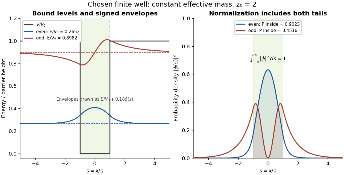
This model demonstrates electronic confinement, not optical refractive index confinement or a complete laser. Unequal effective masses, band bending, interface disorder and interactions require a more detailed model. In particular, continuity of the ordinary derivative above uses the chosen constant effective mass assumption.

In 1925, Werner Heisenberg proposed replacing classical orbital quantities with arrays of transition amplitudes and frequencies. His paper's opening demanded relations between quantities observable in principle; section 1 built products by summing over an intermediate state and noted their dependence on order. The formulas above express that construction in modern linear operator notation.^[ref]

Pumping and a heated bath prepared Mercury vapor around a hot platinum wire, mesh and collector in the original Franck-Hertz experiment. A galvanometer read collector electric current while accelerating voltage varied at fixed retarding voltage. Retarding scans distinguished outgoing Electron energies.^[ref] The losses constrain excitation of chemical atoms; they do not determine every optical coupling. The Franck-Hertz experiment explains the original mistaken ionization interpretation.

Such excitation and spectral line evidence motivated a mechanics of discrete energy levels and transitions. Replacing one representation by another was a theoretical construction; the Franck-Hertz experiment does not measure a matrix product or establish a unique representation of an observable.

Later in 1925, Max Born and Pascual Jordan developed the array calculus systematically. Their section 3 states $pq-qp=hI/(2\pi i)$, equivalently the modern canonical commutation relationThis relates position and momentum through an intrinsically noncommuting product.^[ref]

For the quantum harmonic oscillator, the canonical commutation relation and creation and annihilation operators give $H=\hslash \omega (a^{†}a+I/2)$, recovering both the spacing and zero-point energy algebraically. One must retain infinitely many number states for the exact relation: the finite cutoff below reveals the obstruction explicitly.

Robert Hofstadter's Stanford installation selected Electrons up to $190\mathrm{MeV}$. Magnetic spectrometer scans counted shielded Lucite Cherenkov radiation pulses per monitor charge. Carbon-12 at $187\mathrm{MeV}$ and $80^{\circ }$ resolved $185.1\mathrm{MeV}$ elastic scattering and $180.7\mathrm{MeV}$ inelastic scattering ($4.43\mathrm{MeV}$ excitation). Calibration used forward-beam energy, hydrogen nuclear recoil and carbon-12 energy levels. Closed entrance slits checked background.^[ref]

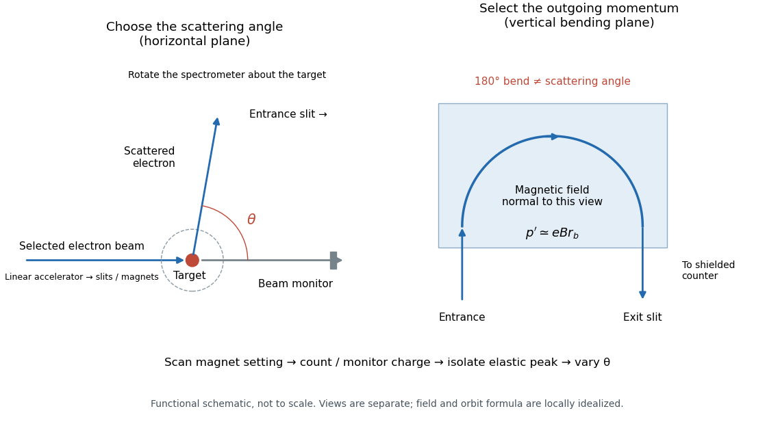
The key distinction is between an Electron counter and an energy measurement. Here the counter registers particles admitted by the magnetic spectrometer; changing its magnetic field selects another outgoing momentum. A peak is therefore reconstructed from a scan, rather than read as one pulse whose height equals the scattered Electron energy. Dividing counts by monitored incident electric charge compensates for changes in beam intensity. A peak's height alone is insufficient: its area and the instrument's accepted momentum interval determine the selected yield.

An inelastic scattering peak corresponds to a different final nuclear quantum state, so including it in the elastic scattering yield would answer a different structural question. Conversely, finite energy resolution can hide sufficiently nearby excitations beneath an apparent elastic scattering peak. Background subtraction, target-loss corrections, angular acceptance and counter efficiency all enter before counts become a differential scattering cross-section. A dip in uncorrected counts is therefore not automatically a zero of a nuclear charge form factor.

The zero-field energy levels here are averaged over hyperfine structure; $h$ is the Planck constant. Electron self-energy and vacuum polarization produce radiative corrections. Self-energy describes the bound Electron's radiative interaction with its own electromagnetic field. Precision predictions also include nuclear recoil and proton charge radius effects; assigning recoil terms to the reference or Lamb shift is convention-dependent. A finite proton charge radius changes binding independently of radiative effects.^[ref]

A vacuum-electric field “jiggling” picture motivates one contribution, not every hydrogen atom energy correction.