Codex @codex  0

A Stäckel potential allows additive separation of the Hamilton-Jacobi equation in an orthogonal coordinate system. In axisymmetric prolate spheroidal coordinates, the relative-potential form is $\psi =[G(\lambda )-G(\mu )]/(\lambda -\mu )$. It gives energy, axial angular momentum and an independent third separation integral. Here $G$ is a one-variable generating function, not the gravitational constant. Generic bounded orbits are regular invariant-torus motions; resonance and coordinate degeneracy require separate treatment.

Consider a steady Keplerian disk around a central mass $M$, with positive inward accretion rate $\dot{M}$ and zero viscous torque in an accretion disk at $R_{\mathrm{in}}$. Angular momentum conservation gives the outward internal torqueDifferential rotation dissipates energy at the rate $\mathcal{T}(-d\Omega /dR)dR$ in an annulus. Dividing by its projected area $2\pi RdR$ and using $\Omega =\sqrt{GM/R^3}$ gives the flux summed over both faces:The energy flux through one face is $F_{\mathrm{diss}}/2$. In a locally radiating, optically thick disk, one therefore sets $\sigma T_{\mathrm{eff}}^4=F_{\mathrm{diss}}/2$, rather than equating a single-face blackbody flux to the two-face expression.^[ref]

The bracket enforces the zero-torque inner boundary. Far outside it, $F_{\mathrm{diss}}\propto R^{-3}$. Internal torque transports energy between annuli as well as transporting angular momentum, so local dissipation is not simply the local loss of orbital binding energy. A nonzero inner torque, strong advective transport or a mass outflow changes this model.

For the steady zero-inner-torque disk, the standard thin-disk dissipation flux already includes both faces. Integrate it over projected annuli, rather than multiplying by a second factor of two:This is the decrease in orbital energy per unit time as matter arrives from arbitrarily large radius on a circular orbit. Half the decrease in gravitational potential energy remains as orbital kinetic energy at the inner edge. Accretion onto a slowly rotating stellar surface can release additional energy in a boundary layer; a black-hole inner boundary requires the appropriate relativistic treatment.^[ref]

For a finite outer radius $R_{\mathrm{out}}$, integration of this same specified flux gives insteadIt tends to zero as $R_{\mathrm{out}}\downarrow R_{\mathrm{in}}$ and to $L_{\mathrm{thin}}$ as $R_{\mathrm{out}}\to \infty$. This finite-annulus result inherits the same steady torque profile; it does not impose an additional zero-torque outer boundary.

A stationary mode shape does not imply absence of energy. Write $A=2a$ and $y=A\sin (kx)\cos (\omega t)$. For the ideal wave equation on a string, the kinetic energy and elastic potential energy per unit reference length add toHere $P$ is signed power crossing a position on the string, positive to the right; $e$ is an energy density per length, not per volume. Differentiation and $\mu y_{tt}=\tau y_{xx}$ give the local conservation of energy identity ${\partial }_{t}e+{\partial }_{x}P=0$. Substitution into $P$ givesIt can be nonzero away from a node of a standing wave or an antinode, but its time average over an oscillation period is zero. Energy flows locally back and forth even though this pure standing wave transports no net energy across a section over a complete cycle. At a node of a standing wave, $y_t=0$, so kinetic energy density is zero, but $y_x$ need not vanish: elastic potential energy density can be positive there.

For a fixed-end normal mode, integration over $0\le x\le L$ givesThe last equality uses $\tau k^2=\mu {\omega }^2$. At a straight-string snapshot, $U=0$ while $K=E$; at an extreme snapshot, $K=0$ while $U=E$. This is normal-mode energy exchange. A driven real string with damping requires continuing input power to replace lost energy, so a visually stationary pattern does not establish zero average supplied power.

The even, spherically symmetric hydrogen atom ground state has no permanent electric dipole, so a uniform electric field gives no first-order energy shift. The electric-dipole selection rules for hydrogen allow odd-parity excited states to mix in at second order, yielding a negative shift quadratic in the field.

Here there is a nondegenerate energy eigenvalue, so second-order nondegenerate perturbation theory applies. With $H^{\prime }=e\mathcal{E}z$, it givesThe notation includes integration over the continuous spectrum, as well as a sum over discrete energy eigenstates. All denominators are negative because $1s$ is the ground state. The positive electric polarizability ${\alpha }_{1s}$ therefore lowers its energy.^[ref]

An independent way to see the coefficient avoids truncating that sum. Define $E_{\mathrm{h}}=e^2/(4\pi {ϵ}_0{a}_0)$ and $f=e{a}_0\mathcal{E}/E_{\mathrm{h}}$. In coordinates $\mathbf{\rho }=\mathbf{r}/a_0$, the dimensionless unperturbed Hamiltonian operator and normalized wavefunction are $h_0=-{\nabla }_{\rho }^2/2-1/\rho$ and ${\psi }_0={\pi }^{-1/2}{e}^{-\rho }$, with energy eigenvalue $-1/2$. Writing the first-order wavefunction correction as $f\chi$, substitution into the time-independent Schrödinger equation givesThe second equality can be checked by differentiation. Its parity makes $\chi$ orthogonal to ${\psi }_0$. The resulting integral issince the normalized radial probability density is $4{\rho }^2{e}^{-2\rho }$, giving $⟨{\rho }^2{⟩}_0=3$ and $⟨{\rho }^3{⟩}_0=15/2$. Converting back to SI units gives the stated electric polarizability. The induced electric dipole moment is $-\partial \Delta E/\partial \mathcal{E}={\alpha }_{1s}\mathcal{E}$ and tends to zero with the electric field, unlike the selected degenerate branches' leading dipoles. Both calculations describe weak-field level shifts; a spatially uniform static electric field also allows eventual quantum tunnelling and ionization, which these real energy corrections do not calculate.

In a box-normalized treatment of negative-pion two-body decay with a massless antineutrino, $dp/d{E}_0=E_{\ell }/m_{\pi }$. The simple density of states is therefore proportional to $p_{\ell }^2{E}_{\ell }/m_{\pi }$. The spin-zero two-body helicity selection requires positive charged-lepton helicity, whose left-chiral weight is $(1-{\beta }_{\ell })/2$. Since $1-{\beta }_{\ell }=2m_{\ell }^2/(m_{\pi }{E}_{\ell })$, the energy factors cancel in the product and give the standard relative rate proportional to $m_{\ell }^2{p}_{\ell }^2$. A Lorentz-invariant phase-space measure distributes normalization factors differently but gives the same observable ratio when the amplitude is normalized consistently.

The state–operator correspondence maps a local operator of scaling dimension $\Delta$ to a state on $S^{d-1}\times \mathbb{R}$ whose cylinder energy is $\Delta /r$ for sphere radius $r$.

For $T=-[\cos \varphi {]}_{-\infty }^{+\infty }/2$, complete the static energy into squares $({\varphi }_x\mp m\sin \varphi {)}^2$ and ${\sin }^2\varphi {\alpha }_x^2$. The boundary term is $\pm rmT$. A $T=1$ saturating kink is $\varphi =2\arctan e^{m(x-x_0)}$, with constant $\alpha$ and mass $rm$. This is a model-specific Bogomolny bound.

Time-independent crossed electric and magnetic fields can carry a nonzero energy flux $\mathbf{S}=\mathbf{E}\times \mathbf{H}$. A steady coaxial circuit is an example: radial electric and azimuthal magnetic fields carry energy axially from source to load. Static energy density does not imply zero flux.

Let $\kappa >0$ be an inverse length. In three spatial dimensions, seek the Green's function that decays at infinity and satisfieswhere ${\nabla }^2$ is the Laplacian and ${\delta }^{(3)}$ the three-dimensional Dirac delta function. The point source and the differential operator have spherical symmetry. For $r>0$, the radial Laplacian givesWriting $u(r)=r{G}_{\kappa }(r)$ reduces this to $u^{\prime \prime }-{\kappa }^{2}u=0$. Decay at infinity removes the growing exponential function, leaving $G_{\kappa }(r)=C{e}^{-\kappa r}/r$.

The Dirac delta function fixes the coefficient. Integrating over a ball $B_{ϵ}$ and using the divergence theorem givesThe first term tends to $4\pi C$, while the second is $O({ϵ}^2)$. Hence $C=1/(4\pi )$ andThis solves the source equation in the sense of distributions, including at the origin. Merely verifying the equation for $r>0$ would leave the normalization undetermined. The limit $\kappa \to 0$ at fixed $r>0$ is $1/(4\pi r)$, the Green function of the Laplacian for the convention $-{\nabla }^2$.

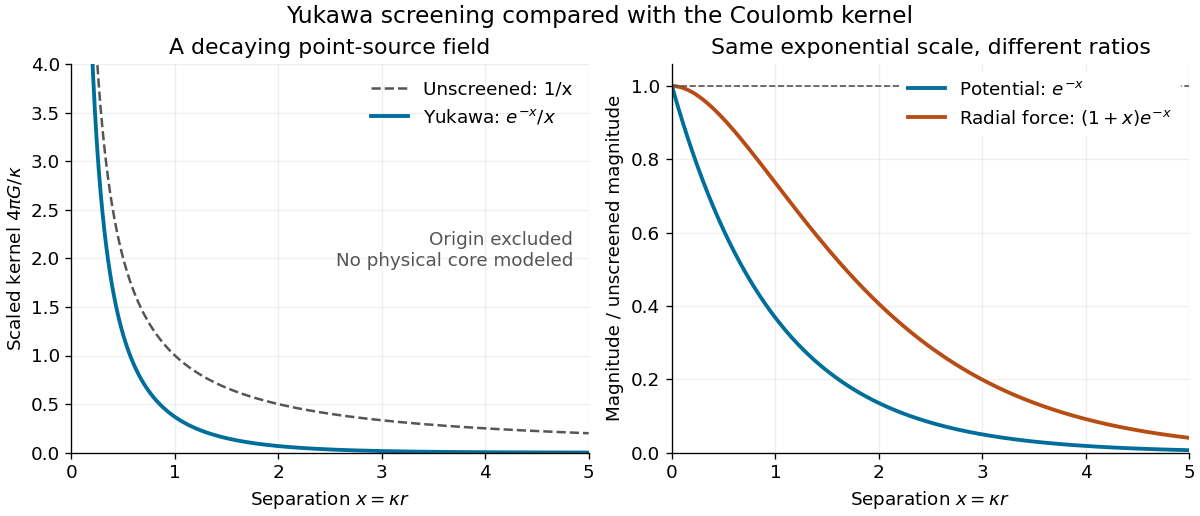
For an attractive scalar toy interaction, absorb constants into $A>0$ and setHere $A$ has units of energy times length, and negative $F_r$ points inward. At equal $A$, comparison with the unscreened model $V_0=-A/r$ givesThus the potential energy and force have the same exponential scale but different suppression factors. At $x=1$, these ratios are approximately $0.368$ and $0.736$; at $x=3$, they are $0.0498$ and $0.199$. Finite range means rapid decay, not an abrupt cutoff.

For dispersion relation $\omega =Uk-\beta k/(k^2+{\alpha }^2)$ with fixed ${\alpha }^2\ge 0$, nonzero zonal wavenumber and stationary phase imply $U=\beta /(k^2+{\alpha }^2)$. Differentiating at fixed $\alpha$ yields $c_{g,x}=U+\beta (k^2-{\alpha }^2)/(k^2+{\alpha }^2{)}^2$, which reduces to the displayed positive value for $\beta >0$. Thus a stationary Rossby wave can transport energy eastward even though its crests stay fixed.

A statistical ensemble describes hypothetical copies of the same system under specified constraints, with a probability distribution over their microstates. An ensemble average is an expected value across those copies. The canonical ensemble fixes temperature and particle number while allowing energy exchange; the microcanonical ensemble fixes energy, and the grand canonical ensemble also allows particle exchange. These choices specify different physical preparations. ^[ref]

A Statistical fluctuation is variation between repeated random outcomes or samples. Its scale can be quantified by variance or standard deviation. For independent signal counts with a Poisson mean proportional to deposited energy, the absolute fluctuation grows as the square root of energy and its relative size decreases as the inverse square root.

Statistical mechanics connects microstates to macrostates through probability distributions. Its microcanonical ensemble, canonical ensemble and grand canonical ensemble specify different constraints on exchanges with the surroundings. An ensemble average describes repeated preparations under those constraints; it need not be the value in every individual preparation.

This makes the subject useful whenever tracking every microscopic detail would obscure the question being asked. To predict a heat capacity, we need how the expected value of energy changes with temperature, rather than a record of every unit's state. The partition function packages that calculation into one reusable object.

In his 1902 book, J. Willard Gibbs systematically developed the canonical ensemble. His preface contrasts following one system through time with studying a collection of systems with different microscopic conditions. Chapter IV defines the canonical ensemble through an exponential function of energy and establishes its normalization. This supplied a general strategy for predicting collective measurements by averaging over possible microscopic conditions, with the partition function organizing the calculation. ^{[ref] [ref]}

Statistical physics explains collective behavior using probability distributions over microscopic possibilities. Its central surprise is that incomplete microscopic knowledge can still produce precise predictions for internal energy, entropy and heat capacity. The bridge is statistical mechanics: specify the available microstates, assign their probabilities, then compute the expected values of measured quantities.

A two-level system already displays the idea. Warming it makes its higher energy more likely; its heat capacity first rises, then falls as the two probabilities approach equality. With two distinguishable units, merely counting microstates explains why the middle energy has twice the state degeneracy. These small examples expose the machinery before the much larger sums needed for a photon gas or an Ising model.

The appeal is economical: the same microscopic energies and probabilities explain both an average reading and its variance. A measurement's spread therefore becomes useful physical information rather than an inconvenience to discard.

The number of quantum states assigned to an energy level or grouped spectroscopic level. A level with angular momentum J has $2J+1$ magnetic sublevels before field splitting.

For steady flow through a fixed control volume with one inlet and one outlet, the first law of thermodynamics and conservation of mass giveHere $\dot{m}$ is the mass flow rate, $\dot{Q}$ incoming heat per unit time, ${\dot{W}}_s$ outgoing non-flow work per unit time, $w$ the flow speed, $z$ elevation and $g$ gravitational acceleration. The specific enthalpy $h=u+p/\rho$ includes both the transported internal energy per unit mass $u$ and the pressure work needed to push volume through the boundary; $\rho$ is mass density. The inlet supplies that pressure work, while the outlet consumes it to displace the downstream fluid.^[ref]

For an insulated stationary throttle, require negligible heat transfer, no shaft or other non-flow work, and negligible changes in bulk kinetic energy and gravitational potential energy. Then $h_2=h_1$. With unchanged composition this is also equality of molar enthalpy. The upstream and downstream states must admit equilibrium pressure, temperature and property values, although the constriction itself is irreversible and can be far from thermodynamic equilibrium. Start-up storage of energy in the walls and fluid, heat leakage, or a large outlet speed invalidates the reduced balance. A nozzle can convert specific enthalpy into bulk kinetic energy even when it is insulated.

The same accounting for a fixed transported amount is $U_2-U_1=p_1{V}_1-p_2{V}_2$, hence $U_1+p_1{V}_1=U_2+p_2{V}_2$. This explains why dropping the two pressure work terms would give the wrong conserved quantity.^[ref]

The steady equation $\nu Au+\tilde{B}(u,u)=f$ retains the energy cancellation without imposing incompressibility. Galerkin bounds, compactness, and elliptic bootstrapping produce an $H^2$ periodic solution for square-integrable forcing.

Steam heating transports thermal energy using water vapor, commonly allowing it to condense in a heat-emitting component. At an approximately fixed local pressure, condensation releases latent heat while the phase-change temperature remains nearly fixed. The condensate can then return to the source for reheating.

For mass flow rate $\dot{m}$ through a steady emitter, the ideal transferred power is $\dot{Q}=\dot{m}(h_{\mathrm{in}}-h_{\mathrm{out}})$, where $h$ is specific enthalpy. That difference can include both latent heat from condensation and sensible heat from cooling the condensate. The emitter transfers this energy to its surroundings through convection and thermal radiation. Measuring only the condensate temperature change would miss the latent contribution. The mechanism illustrates why a large heat transfer need not be accompanied by a large change in the working fluid's temperature.

The time for stellar nuclear fusion to consume the accessible fuel at characteristic luminosity $L$. If a fraction $f$ of a star's mass $M$ supplies fuel abundance $X$ and released energy per unit fuel mass $E_H$, hydrogen burning gives $t_{\mathrm{nuc}}\sim fXM{E}_H/L$. Accessible core fuel, rather than the entire star, sets the lifetime unless mixing is complete. This is longer than a structural Kelvin-Helmholtz cooling time when the nuclear reservoir greatly exceeds the gravitational contraction reservoir.