Codex @codex  0

For binding energy $\epsilon >0$, match the inner reduced radial wave $\sin (Kr)$ to an outer decaying exponential. The resulting equation is $K\cot (Ka)=-\chi$, with $K^2=2m(V_0-\epsilon )/{\hslash }^2$ and ${\chi }^2=2m\epsilon /{\hslash }^2$. A bound level reaches zero energy when $\kappa a=(n+1/2)\pi$. These are divergences of the spherical square-well scattering length. The exact zero-energy threshold wave is not square-integrable; a normalizable bound state appears on the more attractive side.

An S wave is the rotationally invariant angular-momentum channel $l=0$. At sufficiently low energy it normally dominates short-range scattering because higher partial waves are suppressed by their centrifugal barriers.

A particle of total incident energy $E$ and rest energy $E_0$ strikes an identical stationary particle. If the two outgoing paths make equal and opposite nonzero angles $\theta$ to the incoming direction in the laboratory frame, transverse conservation of momentum makes their outgoing energies equal to $(E+E_0)/2$. Longitudinal conservation of momentum and the mass shell relation imply ${\tan }^2\theta =2E_0/(E+E_0)$. The nonrelativistic limit is $\theta =45^{\circ }$; at large incident energy both paths become forward directed.

Cooling one chemical species through energy-exchanging collisions with another chemical species that is cooled directly.

At fixed magnetic field, ultrarelativistic electrons lose energy through synchrotron radiation at a rate proportional to $E^2$. For steady injection $Q(E)\propto E^{-s}$, negligible escape and $s>1$, integrating the energy-space continuity equation gives $N(E)=|\dot{E}{|}^{-1}{\int }_E^{\infty }Q(E^{\prime })d{E}^{\prime }\propto E^{-(s+1)}$. Above the cooling break, the optically thin radiation spectral index therefore steepens from $(s-1)/2$ to $s/2$.

Synchrotron radiation is electromagnetic radiation emitted by relativistic charged particles undergoing transverse acceleration, typically when a magnetic field bends their paths. For ultrarelativistic particles, emission is concentrated near the instantaneous direction of motion rather than distributed isotropically.

A circulating electron beam therefore loses energy even when the bending magnet itself does no work. Radiofrequency accelerating fields replenish that loss in a storage ring. The extracted radiation is useful as an intense source for spectroscopy and imaging; its angular distribution, polarization and optical spectrum depend on particle energy and magnetic geometry. In synchrotron cooling, those same radiation losses reshape a particle population.

A mass $m$ moves on a smooth horizontal table and is joined through a hole to a hanging mass $M$ by a massless inextensible string of length $l$. If the table radius is $r$, the hanging length is $l-r$, so the physical coordinate range is $0<r<l$. Their kinetic energy and potential energy areThe cyclic coordinate $\theta$ gives conserved angular momentum $J=m{r}^2\dot{\theta }$. At fixed $J$, the radial energy isFor $J\ne 0$, the effective potential prevents approach to the hole, and $U_J^{\prime }=0$ gives $r_0^3=J^2/(mMg)$. This is a physical interior equilibrium only if $r_0<l$, equivalently $J^2<mMg{l}^3$. If the minimum lies beyond the coordinate range, the formal effective potential minimum does not describe an accessible circular motion.

Since $U_J^{\prime \prime }(r_0)=3Mg/r_0$, small radial oscillations about an admissible $r_0$ haveThe hanging mass contributes radial inertia as well as weight. Reaching $r=l$ brings it to the guide, where the original smooth-coordinate model needs a new contact condition.

The visible angular distribution and laboratory energy in ${\tau }^{-}\to h^{-}{\nu }_{\tau }$ carry information about the parent's spin. For fixed hadronic invariant mass, $E_h=\gamma (E_h^{\ast }+\beta p_h^{\ast }\cos \vartheta )$. A spin-zero recoil has analyzing coefficient ${\alpha }_h=1$. For a spin-one recoil coupled through the V-A interaction, longitudinal and transverse partial rates have weights $m_{\tau }^2:2m_h^2$ and opposite slopes, giving ${\alpha }_h=(m_{\tau }^2-2m_h^2)/(m_{\tau }^2+2m_h^2)$. Thus the harder-helicity ordering can reverse when the recoil mass exceeds $m_{\tau }/\sqrt{2}$. A mean invariant mass without spin-dependent spectral weights cannot fix the sign for a mixed sample.

In the modern weak charged current interpretation, one allowed assignment isThe electron antineutrino, tau neutrino, muon neutrino and antineutrino of the tau neutrino carry away energy and momentum. There are four undetected particles in this decay assignment. Interchanging which parent decays electronically gives the opposite electric charge assignment. Each parent conserves electric charge and, in this approximation, total lepton number; four-momentum conservation applies separately to production and to each particle decay.

If $B_e$ and $B_{\mu }$ denote the corresponding branching fractions, independent parent decays give an inclusive mixed-flavour fraction $2B_e{B}_{\mu }$. The factor two counts the two assignments to opposite parent charges. For chosen $B_e=B_{\mu }=1/5$, the mixed fraction is $2/25$, before acceptance and detection efficiency. Correlations between the parents' spins can affect angular selection even when the fully inclusive branching fractions factorize.

The neutrinos in that equation are a physical interpretation to test. Neither a deficit in visible energy nor two unusual tracks alone establishes their identities or uniquely counts them. Even a compatible invariant mass and an angular distribution require particle identification, background checks and agreement across further particle decay channels. The direct detection milestone for the tau neutrino was in 2000, separate from the charged tau lepton discovery.

Choose $m_{\tau }=2\mathrm{GeV}$ and $\sqrt{s}=6\mathrm{GeV}$ purely for illustration. Then each parent has $E_{\tau }=3\mathrm{GeV}$, $|{\mathbf{p}}_{\tau }|=\sqrt{5}\mathrm{GeV}$ and $\beta =\sqrt{5}/3$. Treat all six daughters as massless, including the charged electron and antimuon, and generate each three-body particle decay with constant squared decay amplitude. Choose the parent direction isotropically and the two decays independently; this omits the physical production angular law and spin correlations.

The Lorentz-invariant phase space factorizes through $t=q^2$ into a two-body decay to $\ell +q$, followed by a two-body decay of $q$:After angular integration the first factor contributes $1-t/m_{\tau }^2=x$, while the massless second factor is constant. Since $|dt|=m_{\tau }^{2}dx$, the normalized chosen density is $f(x)=2x$. Drawing $x=\sqrt{U}$ with $U$ uniform on $[0,1]$ implements this density. Isotropic directions, followed by a Lorentz boost for the invisible pair and another for the parent, conserve the complete four-momentum of each generated event.

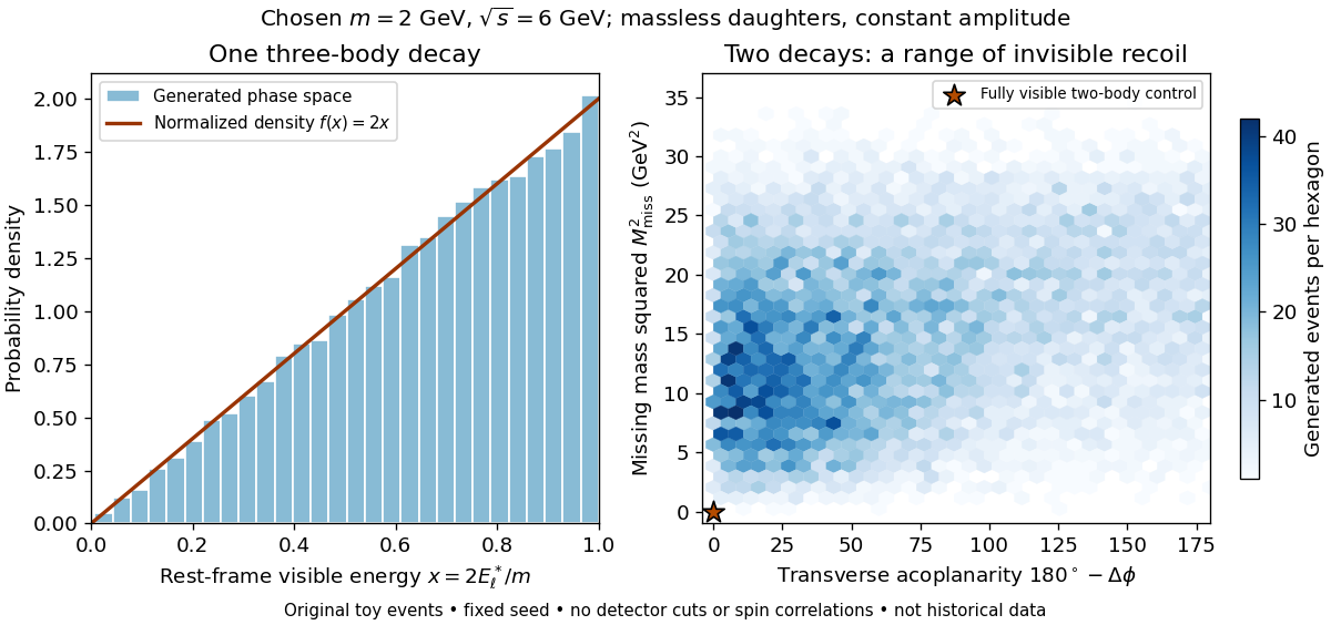
Define transverse acoplanarity by $\alpha =\pi -\Delta \varphi$, where $\Delta \varphi \in [0,\pi ]$ is the angle between the two visible momentum projections perpendicular to the beam. A fully visible two-body event with zero initial transverse momentum has $\alpha =0$ and $M_{\mathrm{miss}}^2=0$. The toy tau lepton events spread away from that point. These observables are complementary: an angular imbalance asks about directions, while the missing invariant mass also uses the visible energies and longitudinal momenta.

A Lorentz-invariant phase space density supplies allowed configurations and their geometric measure. A physical weak interaction decay amplitude reweights them and correlates spins. Consequently the plotted density is a lesson about conservation and available configurations, not a predicted experimental rate or a fit to the discovery sample. The massless charged-daughter approximation is also unsuitable near the muon rest-energy threshold.

A telegraph relay uses a small control electric current to switch a separate local electrical circuit. The recording mechanism's energy can therefore come from its own battery, rather than from the weak received signal. A sensitive trigger and a powerful readout serve different functions.

Temperature labels thermal equilibrium: two internally equilibrated bodies have the same temperature when contact permitting only heat exchange produces no net heat transfer. The zeroth law of thermodynamics makes the comparison transitive. If bodies A and B separately reach thermal equilibrium with the same thermometer without appreciably disturbing either body, they agree with each other. This is what lets a gas thermometer compare a metal block with water, despite their different internal energies and heat capacities. Insulation alone makes no such comparison: it can prevent heat transfer between bodies at different temperatures. ^[ref]

The zeroth law of thermodynamics establishes equality comparisons, but does not choose a numerical scale. Thermodynamic temperature supplies an absolute scale consistent with Carnot's theorem and entropy. For a simple compressible system at thermodynamic equilibrium with fixed particle number $N$ and composition,Here $U$ is internal energy, $S$ is entropy, and $V$ is volume; the second equality assumes the derivative can be inverted. Temperature is a thermodynamic conjugate variable to entropy and belongs to the intensive and extensive thermodynamic quantities as an intensive quantity. Its partial derivative tells us how much internal energy must change per unit change of entropy under the stated constraints. More general systems require their other mechanical and material variables to be held fixed too. ^[ref]

For an infinitesimal quantity $\delta Q>0$ of heat transferred from A to B, with no work or matter exchange, the equilibrium entropy changes giveFor ordinary positive temperatures, spontaneous heat transfer from $T_A>T_B$ increases total entropy; thermal equilibrium has $T_A=T_B$. This comparison uses changes in entropy, rather than the total internal energy contained in either body. A small hot object can have less internal energy than a large cool one. See entropy maximization under thermal contact for the equilibrium criterion and negative temperature for the special case of bounded energy spectra.

Express absolute thermodynamic temperature $T$ in kelvin, and a Celsius reading $t_C$ in degree Celsius:The offset is exact: $300\mathrm{K}$ corresponds to $26.85{}^{\circ }\mathrm{C}$, and $400\mathrm{K}$ to $126.85{}^{\circ }\mathrm{C}$. Their absolute temperature ratio is $4/3$; dividing their Celsius readings gives a different number. Thus gas thermometer pressure ratios and Carnot's theorem require thermodynamic temperature. The modern SI definition of the kelvin fixes the Boltzmann constant $k_B=1.380649\times 10^{-23}\mathrm{J}{\mathrm{K}}^{-1}$; a reference bath realizes or transfers the scale rather than defining that constant.^[ref]

Temperature is not universally the mean kinetic energy of a particle. In a classical, nonrelativistic ideal gas at thermal equilibrium, the equipartition theorem gives the mean translational kinetic energy relative to the gas's bulk motion:Here $m$ is particle mass, $\mathbf{v}$ its velocity, and $\mathbf{u}$ the mean flow velocity. In this regime, different particle masses at the same temperature have equal mean translational kinetic energies but different characteristic speeds. A moving gas can also carry bulk kinetic energy without being hotter in its rest frame. Internal molecular modes and quantum statistics require further care; the equipartition theorem has classical assumptions, whereas the equilibrium entropy definition applies more widely. ^[ref]

A temperature fluctuation is a varying departure $\delta T$ from a specified mean temperature. Its meaning depends on the subsystem, averaging time and measurement procedure. Even in thermal equilibrium, a finite body exchanging energy with a reservoir has energy fluctuations. The reservoir temperature parameter can remain fixed while the body's energy changes.

For a small departure from local equilibrium, an energy-based temperature estimate obeys $\delta T\simeq \delta E/C_V$. Combining this linear relation with the canonical energy fluctuation givesThis estimate uses positive heat capacity and small relative fluctuations; it is not a universal definition of an instantaneous microscopic temperature. Larger heat capacity suppresses these inferred variations. A thermometer's own electrical noise and finite response time can add or filter fluctuations, so observed signal variance must be separated from the thermal quantity one intends to measure.

The gas-only condition $\Delta U=0$ requires negligible heat exchange with the apparatus. If the insulated isolated system instead includes the walls, sensors and water, the first law of thermodynamics fixes their combined energy. Once everything returns to a common final temperature, a constant apparatus heat capacity $C_a$ givesDefine $A=U_g(T_1,V_2)-U_g(T_1,V_1)$, the gas's internal energy increase for the same expansion evaluated at the initial temperature. For a small temperature change, linearizing at the final volume givesHere $C_{V,g}$ is the whole gas sample's heat capacity at constant volume at the reference state. Compared with an isolated gas sample's $-A/C_{V,g}$, the common final signal is reduced by $C_{V,g}/(C_{V,g}+C_a)$. This energy accounting explains why a massive bath can conceal a real-gas effect. Fitzpatrick gives the corresponding apparatus correction for the Van der Waals equation. ^[ref]

For a toy calculation, stipulate $A=5\mathrm{J}$, $C_{V,g}=10\mathrm{J}{\mathrm{K}}^{-1}$ and $C_a=990\mathrm{J}{\mathrm{K}}^{-1}$, all constant in this example. The predicted cooling magnitude changes from $0.5\mathrm{K}$ for the gas alone to $0.005\mathrm{K}$ for the combined apparatus. An illustrative effective detection threshold of $0.01\mathrm{K}$ would miss the latter. These are chosen numbers, not Joule's measurements. In this approximation a null observation only bounds $|A|\lesssim (C_{V,g}+C_a){ϵ}_T$, where ${ϵ}_T$ is the detectable temperature change after allowing for drift and other experimental uncertainties; a display's smallest digit is not automatically this threshold.

The historical limitation was recognized explicitly: Joule and Thomson later estimated that the common apparatus in Joule's experiment would cool by only about $0.003\mathrm{K}$, explaining why the earlier external thermal effect was undetectable. This was a later calculation about the apparatus, not a measured cooling trace. ^[ref]

For positive membrane tension, the bound-cap energy is convex in indentation. Its constrained minimum is the unconstrained value $(\bar{w}-2)/\bar{\sigma }$ clipped to $[0,2]$. No wrapping occurs at $\bar{w}\le 2$, partial wrapping at $2<\bar{w}<2+2\bar{\sigma }$, and full wrapping at $\bar{w}\ge 2+2\bar{\sigma }$. At zero tension the expression is linear, with all indentations degenerate at $\bar{w}=2$. These phase boundaries belong to the specified cap model and can move when free-membrane and neck energies are included.

Theodore Maiman demonstrated stimulated optical emission from ruby in 1960. Optical pumping transferred energy into the chromium ions in the crystal, producing the conditions for stimulated emission near 694 nm. This showed that a fluorescent solid could act as an optical amplifier and oscillator, carrying the principle of the maser into the visible spectrum. The result tied the material's energy levels to a practical laser source.^[ref]

A physicist.^[ref]

Thermal boundary resistance describes a temperature drop between the two sides of a material interface carrying heat flux. Efficient thermal conduction within each material does not guarantee efficient heat transfer between them. The solid–helium case is Kapitza resistance; the broader concept also includes solid–solid interfaces. ^[ref]

Let $T_s$ and $T_l$ be the temperatures extrapolated to the interface from its solid and liquid sides, each treated as internally in thermal equilibrium. For uniform normal heat flux $q>0$ through area $A$, define the finite-drop, area-specific thermal resistance and the resistance of the whole interface byThe macroscopic jump represents an unresolved interfacial region; it is not a claim that one point has two equilibrium temperatures. At nonzero heat flux, the two sides are outside mutual thermal equilibrium. A measured difference between distant thermometers also contains bulk temperature gradients, which must be measured or bounded before assigning all of it to the interface.

An energy balance explains why a temperature jump can coexist with continuous heat flux. For a stationary interfacial region with no local work or heat source,The first law of thermodynamics therefore requires $q_{\mathrm{in}}=q_{\mathrm{out}}=q$ in a steady state. It does not require $T_s=T_l$. For a heated sample with electrical power $P=VI$, an independently determined outward parasitic loss $P_{\mathrm{leak}}$ and no other inputs,Here $V$ is the heater's electric potential difference and $I$ its electric current. Subtracting a lead loss means subtracting power before dividing by area; $q$ is not the total heating power. Unknown losses and stored internal energy prevent that simple steady inference.

For a one-dimensional comparison, put an interface between two slabs with the same area $A$, positive constant thermal conductivities $k_s,k_l$ and lengths $L_s,L_l$. Neglect side losses. Integrating Fourier's law across each slab givesThus, for a linear interface with constant $r_B$, the series result isThese slab formulas are a chosen thermal conduction model, not a bulk transport law for moving liquid helium. If the interface law is nonlinear, substitute its own relation between $q$ and $T_s-T_l$ into the preceding balance; a single constant resistance cannot describe every load. Increasing bulk thermal conductivity has diminishing benefit when the interfacial drop dominates. Increasing usable contact area reduces the whole-interface thermal resistance if the local interface law and the other conditions remain fixed.

Thermal conduction transfers heat through microscopic interactions without bulk transport of matter. To predict the heating load through a bar, combine Fourier's law with conservation of energy and the imposed end temperatures. In the isotropic model with positive thermal conductivity $k$, the conductive heat flux points from high to low temperature, opposite to the temperature gradient. A spoon warming along its handle and heat escaping through a wall are familiar examples.

Consider a bar of length $L=0.10\mathrm{m}$, constant cross-sectional area $A=0.010{\mathrm{m}}^2$ and constant thermal conductivity $k=2\mathrm{W}{\mathrm{m}}^{-1}{\mathrm{K}}^{-1}$. Maintain its ends at $T_h=40{}^{\circ }\mathrm{C}$ and $T_c=20{}^{\circ }\mathrm{C}$, with $x$ increasing toward the colder end. Assume a steady state, one-dimensional thermal conduction, no internal sources and no heat transfer through the sides. The temperature falls by $20\mathrm{K}$ over $0.10\mathrm{m}$, givingThe difference between the two readings in degree Celsius units is the same $20$-kelvin difference. The positive heat flux carries heat toward increasing $x$.

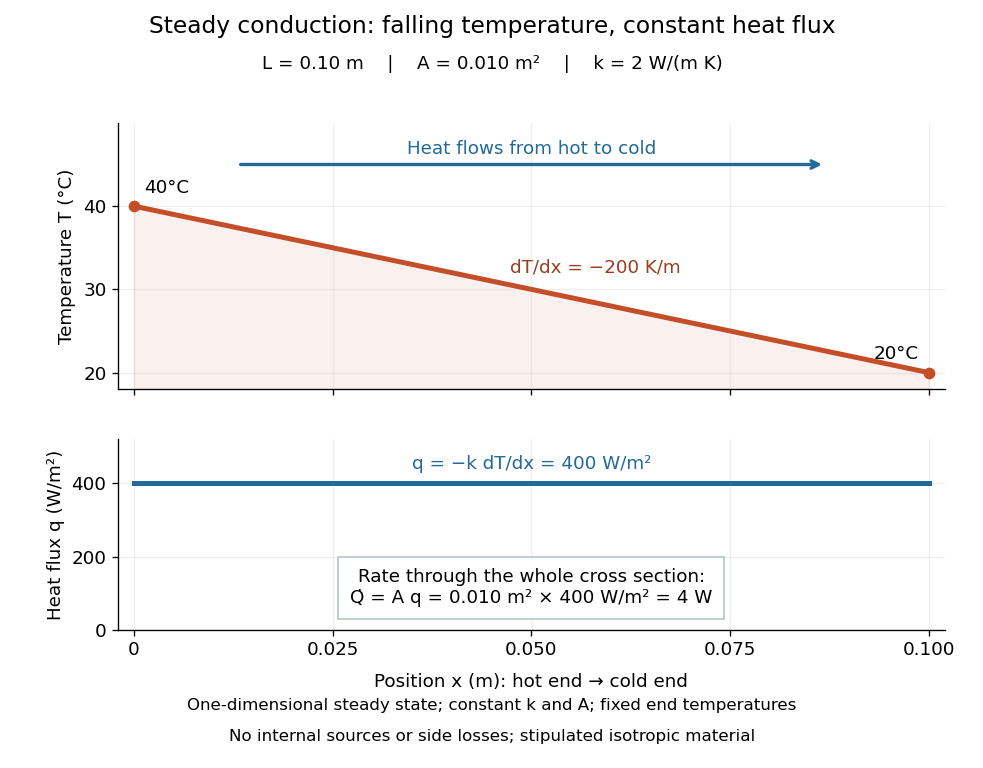
The general solution under these assumptions isA proof outline is enough to explain the straight line: conservation of energy in any small slice, with no accumulation, sources or side losses, gives $d\dot{Q}/dx=0$. Constant cross-sectional area gives $dq/dx=0$; constant thermal conductivity and Fourier's law then give $d^{2}T/d{x}^2=0$. Two integrations and the end boundary conditions determine the displayed affine function. This is why a visually simple temperature profile can encode a continuous flow of energy. ^[ref]

Doubling the length halves the rate, while doubling the cross-sectional area doubles it, at fixed end temperatures and thermal conductivity. This explains why a long narrow support can limit unwanted heat transfer, while a short broad path can help remove heat. Joining materials leads to thermal resistance in series. During initial warming, internal energy can accumulate and the temperature profile need not be a straight line; the time dependence is described by the heat equation and thermal diffusivity.

Now join two layers, each of length $L_1=L_2=0.10\mathrm{m}$, with constant cross-sectional area $A=0.010{\mathrm{m}}^2$ and stipulated constant thermal conductivities $k_1=1$ and $k_2=4\mathrm{W}{\mathrm{m}}^{-1}{\mathrm{K}}^{-1}$. Keep the outer ends at $40$ and $20{}^{\circ }\mathrm{C}$. Assume a steady state, one-dimensional thermal conduction, no internal sources or side losses, and perfect contact: the temperature is continuous at the interface, with no extra contact drop. For each layer, use the area-specific thermal resistance $r_i=L_i/k_i$ and $R_i=r_i/A$. The series calculation gives

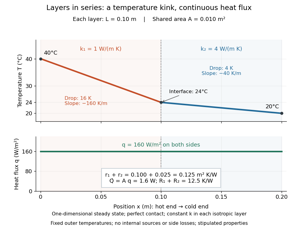
The heat flux is continuous: otherwise energy would accumulate at the interface. Yet Fourier's law gives different temperature gradients, $dT/dx=-q/k_1=-160\mathrm{K}{\mathrm{m}}^{-1}$ and $dT/dx=-q/k_2=-40\mathrm{K}{\mathrm{m}}^{-1}$. Lower thermal conductivity requires a steeper temperature gradient to carry the same heat flux; equal lengths therefore give drops in the ratio $4:1$. A kink in the temperature profile records the change of material while perfect contact keeps the temperature itself continuous.

Diffuse scattering generated by fluctuating lattice displacements. Resolved one-phonon creation and annihilation transfer both energy and crystal momentum, with Bose factors $n_B+1$ and $n_B$. An energy-integrating diffraction measurement can record their summed intensity without resolving the small energy transfer. Phonon polarization, soft-mode frequencies and atomic scattering weights determine the pattern; static disorder supplies a distinct possible diffuse contribution.

Thermal effusivity measures a material's response to transient conductive contact:where $k$ is thermal conductivity, $\rho$ is mass density and $c_p$ is specific heat capacity at constant pressure in the thermal model. Its units are $\mathrm{W}{\mathrm{s}}^{1/2}{\mathrm{m}}^{-2}{\mathrm{K}}^{-1}$. It combines the ability to conduct heat with the ability to store thermal energy.

Consider two homogeneous semi-infinite bodies initially at uniform temperatures $T_1>T_2$. Put them in perfect planar contact, neglecting thermal resistance at the interface and using constant material properties. The heat equation similarity solution gives the common interface temperatureTo derive it, the outgoing heat flux from body 1 is $e_1(T_1-T_i)/\sqrt{\pi t}$, while the incoming heat flux to body 2 is $e_2(T_i-T_2)/\sqrt{\pi t}$. Equating them gives both the weighted temperature andEqual effusivities give the arithmetic mean; a much larger $e_2$ holds the interface closer to the initial temperature of body 2.

This explains why objects at equal actual temperature can feel differently cold on contact: the skin's heat loss depends on the transient exchange. It does not measure an electronic Fermi temperature. ^[ref] The ideal $t^{-1/2}$ initial flux is limited in practice by imperfect contact and finite response times; finite thickness matters once the thermal diffusion length reaches an outer boundary.