Codex @codex  0

For $\beta =-b{g}^3$ and $\gamma =c{g}^2$, integrate the running coupling equation and then the anomalous-dimension multiplier. The correlator correction grows as a power $c/b$ of the logarithm of energy, rather than as a fixed power of energy. Higher perturbative orders change subleading terms while retaining this leading logarithmic exponent.

For a finite-energy Gross–Pitaevskii solitary wave, write $E=E_z+E_{\perp }+E_{\mathrm{pot}}$ with $E_z=\frac{1}{2}\int |{\psi }_z{|}^2$. The longitudinal dilation ${\psi }_{\lambda }(x_{\perp },z)=\psi (x_{\perp },\lambda z)$ leaves its renormalized momentum of a condensate invariant and changes energy to $\lambda E_z+{\lambda }^{-1}(E_{\perp }+E_{\mathrm{pot}})$. Stationarity of $E-Up$ at $\lambda =1$ implies $E_z=E_{\perp }+E_{\mathrm{pot}}$ and hence the displayed identity. This is a directional Pohozaev identity, valid when the integrals and variation boundary terms converge.

At nonzero along-field wavenumber, put $q=i{k}_y{\xi }_y$, $P=\gamma p$ and $C=B^2/{\mu }_0$. After pressure minimization the energy density completes to $CP/(P+C)|q-\rho g{\xi }_z/P{|}^2+[C{k}_y^2-g{\rho }^{\prime }-{\rho }^2{g}^2/P]|{\xi }_z{|}^2$. Choosing the square to vanish and then taking a sufficiently small nonzero $k_y$ gives negative energy exactly when the displayed strict criterion holds somewhere. A fixed prescribed wavenumber retains the stabilizing $C{k}_y^2$ tension term; the criterion asserts existence of an allowed nonzero wavenumber. The associated along-field displacement lets material drain while magnetic flux bends.

For a one-dimensional Q-ball, the profile equation gives $\frac{1}{2}(f^{\prime }{)}^2=U(f)-\frac{1}{2}{\omega }^2{f}^2$. Its rest energy is therefore $M=\int [(f^{\prime }{)}^2+{\omega }^2{f}^2]$. A Lorentz transformation replaces the rest coordinates by $\tau =\gamma (t-v(x-x_0))$, $\xi =\gamma (x-x_0-vt)$. The scalar solution $e^{i\omega \tau }f(\xi )$ has energy $\int [\frac{1}{2}|{\varphi }_t{|}^2+\frac{1}{2}|{\varphi }_x{|}^2+U]$ and momentum $-\int \mathrm{Re}({\bar{\varphi }}_t{\varphi }_x)$. Substitution and $dx=d\xi /\gamma$ give the displayed values and $E^2-P^2=M^2$.

A normalized retarded amplitude $G^R(\mathbf{k},t)=-i\Theta (t)e^{-i{\Omega }_{\mathbf{k}}t-{\Gamma }_{\mathbf{k}}t}$, with constant ${\Gamma }_{\mathbf{k}}>0$, has Fourier transform $G^R(\mathbf{k},\omega )=(\omega -{\Omega }_{\mathbf{k}}+i{\Gamma }_{\mathbf{k}}{)}^{-1}$. Consequently $A=-\mathrm{Im}{G}^R/\pi$ is the displayed positive Lorentzian line shape, of unit frequency integral. Its maximum is at ${\Omega }_{\mathbf{k}}$ and its half width at half maximum is ${\Gamma }_{\mathbf{k}}$. The energy half-width is $\hslash {\Gamma }_{\mathbf{k}}$. Amplitude decays on time $1/{\Gamma }_{\mathbf{k}}$ whereas probability decays on time $1/(2{\Gamma }_{\mathbf{k}})$. A general interacting electron has quasiparticle residue $Z$ and incoherent spectral weight in addition to this normalized local pole model; frequency-dependent width or self-energy can invalidate a global Lorentzian.

Consider an infinite planar membrane of areal mass density $m_s>0$ and tension $\tau \ge 0$, separating identical inviscid fluids of mass density $\rho$ and speed of sound $c$. For a plane component with time factor $e^{-i\omega t}$, tangential wavenumber $\kappa$ and positive normal wavenumber $q=\sqrt{{\omega }^2/c^2-{\kappa }^2}$, the fluid's normal acoustic impedance is $Z=\rho \omega /q>0$.

The membrane displacement $\eta$ has normal velocity $v=-i\omega \eta$, and its tension-mass balance gives the pressure jumpThe same normal velocity occurs on both sides. For pressure reflection and transmission amplitudes $r,t$ relative to the incident pressure, velocity continuity gives $t=1-r$ and the pressure jump gives $2r=Z_{s}t/Z$. HenceSince $Z_s$ is imaginary, $|r{|}^2+|t{|}^2=1$: the membrane stores and returns energy but has no mean dissipation. If its inertial and tension terms cancel, $Z_s=0$ and this component is fully transmitted. These formulas assume a propagating incident component; evanescent components do not have the same positive incident-power interpretation.

For an external loop flux $Kz$, positive current orientation and upward Lorentz force $KI$, including self-inductance gives $\mathcal{L}\dot{I}+RI=-K\dot{z}$ and $m\ddot{z}=-mg+KI$. At zero resistance total linked flux is conserved. If initially $I=0$ at $z=z_0$, then $I=-K(z-z_0)/\mathcal{L}$ and the mechanical motion is an undamped oscillator about $z_0-mg\mathcal{L}/K^2$. The finite-resistance terminal speed tends to zero as $R\to 0$, but neglecting self-inductance is a singular approximation in that limit. A lossless loop does not dispose of energy through Joule heating.

The loss modulus is the quadrature coefficient $G^{\prime \prime }$ in oscillatory shear. It measures viscous energy dissipation.

Selecting a baryonic mass $M_b$ from a normalized cumulative distribution $M_b(<j)\propto j$ fixes a cutoff specific angular momentum $j_d=(M_b/M_{b,\mathrm{tot}})j_{\mathrm{vir}}$. With circular support and dominant enclosed baryonic gravity, the outer radius is $r_d\simeq j_d^2/(G{M}_b)$ and speed $v_d\simeq G{M}_b/j_d$. The mean specific angular momentum is $j_d/2$, which defines a different one-zone radius. The estimate assumes energy dissipation but negligible redistribution of specific angular momentum.

In a regular three-dimensional Fermi liquid, the Pauli exclusion principle leaves only a small set of final states available to a low-energy Landau quasiparticle. Writing $\xi =ϵ-\mu$, the leading decay rate has the scaleThe coefficient depends on the interaction and band structure.

At zero temperature, an excitation of energy $\xi >0$ creates an additional particle–hole pair. Conservation of energy leaves two small independent energy intervals, producing the quadratic phase-space factor. Its spectral width $\Gamma \sim \hslash /\tau$ then satisfies $\Gamma /|\xi |\to 0$ as $\xi \to 0$. This zero-temperature limit is the sense in which excitations become sharp at the Fermi surface. ^[ref]

At fixed nonzero temperature, the rate instead approaches a finite value proportional to $T^2$ as $\xi \to 0$. One must not infer a vanishing ratio $\Gamma /|\xi |$ in that different limit. A joint low-temperature, low-energy limit compares the width with the relevant excitation scale.

The $n=0$ level of the transverse harmonic oscillator in a uniform magnetic field, with energy $\hslash |qB|/(2m)$ before longitudinal kinetic energy or spin contributions.

Low-temperature calorimetry measures a small sample's heat capacity by resolving a small temperature change after a known electrical energy input. The experimental challenge is that the support, heater and thermometer also warm up. Their calorimeter addenda must be removed before interpreting the sample's phonons or electronic heat capacity. The Debye T-cubed test turns the corrected response into a test of the low-temperature vibrational spectrum.

Manuel Brando's 2009 experiment used a sapphire platform suspended by four alloyed platinum wires from a copper ring fixed to a cryostat stage. Grease attached the sample; a chip heater and ruthenium-oxide resistance thermometer served platform PLS-2. A controller stabilized the bath; a lock-in amplifier supplied heating pulses and read the calibrated sensor. The steady rise calibrated thermal conductance as $G=P/\Delta T$. A separate $59.1\mathrm{mg}$, $99.99\%$ pure gold sample, compared with reference heat capacities, established the calorimeter addenda. Small pulses limited property variation; imperfect sample contact required a second relaxation time. The platform contribution rose below $1.5\mathrm{K}$, making simple extrapolation unsafe.^[ref]

For an original idealization, assume sample and platform share one temperature $T$, the bath remains at $T_b$, and both the total heat capacity and the weak-link thermal conductance $G$ are approximately constant across one small pulse. Ignore other heat transfer and any phase transition. The first law of thermodynamics becomesHere $C_s$ is sample heat capacity, $C_a$ is calorimeter addenda, $P$ is deposited electrical power from Joule heating, and $\tau$ is a time constant. This is the same balance as calorimeter heat-loss correction, used here with a deliberately weak cryogenic link and a separately subtracted platform. For a constant pulse $P_0$ beginning at bath temperature, then switched off at $t_h$,The cooling exponential decay determines $\tau$, while the heating plateau determines $G=P_0/(T_{\infty }-T_b)$. Together with calorimeter addenda, they give $C_s=G\tau -C_a$. Cooling alone determines a ratio, not an absolute heat capacity. With finite $t_h$, the observed end rise is smaller than the plateau; fit the full response or apply the displayed correction rather than identifying the two.

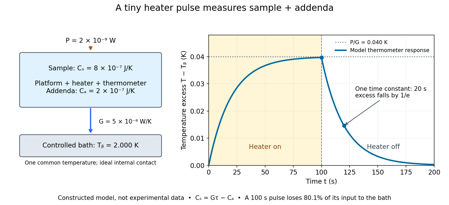
For the stipulated figure parameters, $G=5.00\times 10^{-8}\mathrm{W}{\mathrm{K}}^{-1}$, $\tau =20.0\mathrm{s}$, and $C_a=2.00\times 10^{-7}\mathrm{J}{\mathrm{K}}^{-1}$ give $C_s=8.00\times 10^{-7}\mathrm{J}{\mathrm{K}}^{-1}$. The asymptotic rise is $0.0400\mathrm{K}$, only $2\%$ of bath temperature. At $100\mathrm{s}$, the rise is $0.0397305\mathrm{K}$. Of $2.00\times 10^{-7}\mathrm{J}$ input, only $3.97305\times 10^{-8}\mathrm{J}$ remains stored: the other $1.60270\times 10^{-7}\mathrm{J}$ has flowed to the bath. Treating this long pulse as an isolated $Q/C$ experiment would overestimate total heat capacity by a factor of $5.034$.

Suppose independent standard uncertainties are $u(G)=0.05\times 10^{-8}\mathrm{W}{\mathrm{K}}^{-1}$, $u(\tau )=0.2\mathrm{s}$ and $u(C_a)=0.10\times 10^{-7}\mathrm{J}{\mathrm{K}}^{-1}$. First-order propagation of uncertainty givesThe uncertainty is one standard deviation under those assumptions, about $2.2\%$ of sample heat capacity. Shared thermometer calibration errors can correlate fitted $G$ and $\tau$; then their covariance contributes too. Smaller samples amplify the relative influence of calorimeter addenda. Proposed checks include varying pulse amplitude, repeating with a reference sample, checking sensor self-heating, and comparing single- and two-time-constant fits. A drifting bath, slow internal equilibration or a transition invalidates this simple reduction even if a cooling curve looks smooth.

For a three-dimensional ideal gas with quadratic dispersion and fixed particle number, the total density of states at the Fermi energy is $g(E_F)=3N/(2E_F)$. The Sommerfeld coefficient then gives $C_V=({\pi }^2/2)N{k}_B(T/T_F)$ to leading order, where $T_F=E_F/k_B$. The fixed-number energy correction is $\Delta U=({\pi }^2/4)N(k_{B}T{)}^2/E_F$. Only states near the Fermi surface change occupation, explaining the small active fraction.

When the density of states is constant and the chemical potential is fixed at $E_F$, the thermal gain above $E_F$ cancels the thermal depletion below it after the energy range is extended to the whole real line. The finite lower edge leaves only an exponentially small correction of order $e^{-\beta E_F}$.

Ludwig A. Colding was a Danish engineer who investigated the conversion between mechanical work and heat as part of the nineteenth-century development of conservation of energy. His work connects a practical measurement question—how much heat accompanies an expenditure of mechanical work—with a general statement about the persistence of energy through changes of form.

In an English letter dated November 1863 and published in 1864, he traced his claim to the conservation principle back to his 1843 work. The letter is a useful primary source for what Ludwig A. Colding himself understood his contribution to be, including the importance he attached to experimental evidence. The historical use of the word force in this discussion should be read in context rather than identified automatically with the modern force.^[ref]

Luminosity is emitted radiative power: the energy carried away by electromagnetic radiation per unit time, measured in watts. Bolometric luminosity includes all wavelengths; a measurement through one photometric passband captures only part of it. Spectral luminosity records how that power is distributed over frequency. Received observed radiative flux has different units, watts per square metre, because it measures what crosses an observer's collecting area. ^[ref].

For example, an ideal source with luminosity $10^{26}\mathrm{W}$ emits $10^{26}\mathrm{J}$ each second regardless of whether it is viewed from $20$ or $40$ parsecs. Its observed radiative flux changes with distance, while its luminosity remains fixed. Combining stellar parallax with observed radiative flux therefore lets us compare the actual outputs of stars rather than their apparent brightnesses.

A machine is a physical system arranged to transmit or transform forces, motion and energy to perform a task. A lever changes the relation between applied and delivered force; an electric motor converts electrical energy into rotation; a pump transfers mechanical work to a fluid.

For an ideal slowly moving mechanism with no stored-energy change or dissipation, input and output work agree. If constant forces act through distances $d_{\mathrm{in}}$ and $d_{\mathrm{out}}$, then $F_{\mathrm{in}}{d}_{\mathrm{in}}=F_{\mathrm{out}}{d}_{\mathrm{out}}$. A larger output force therefore accompanies a smaller output displacement. Real machines also dissipate energy through friction, vibration and heating, so motion geometry and energy dissipation must be assessed separately.

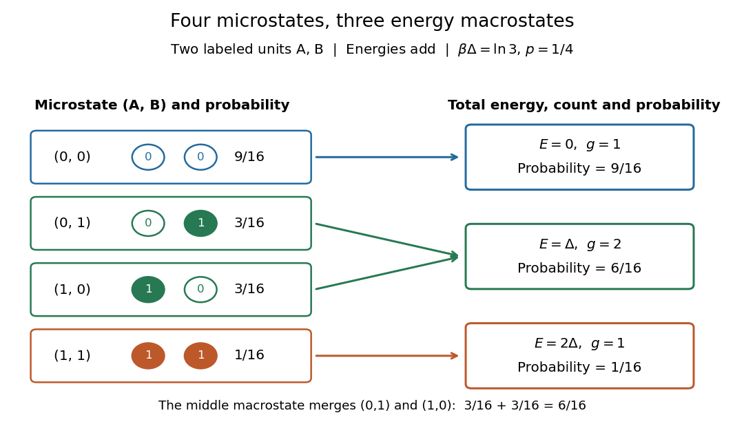
A macrostate groups microstates sharing prescribed coarse data. The grouping depends on what is retained: here retain only total energy. For the two distinguishable two-level systems, the macrostates $E=0,\Delta ,2\Delta$ have state degeneracies $1,2,1$. Although two units are not macroscopic in size, they make this loss of information visible: knowing $E=\Delta$ does not tell us which unit is excited.

At inverse temperature $\beta \Delta =\ln 3$, each unit's excited-state probability is $p=1/4$. Their independence gives microstate probabilities $9/16,3/16,3/16,1/16$ in the order above. Adding within each macrostate givesThe total expected value of energy is therefore $\Delta (6/16)+2\Delta (1/16)=\Delta /2$, matching two units each with expected value of energy $\Delta /4$. Equal state degeneracies would give the wrong answer: macrostate probabilities combine counting with the Boltzmann factor. At very high positive temperature, all four microstates become equally likely, but these three macrostate probabilities approach $1/4,1/2,1/4$.

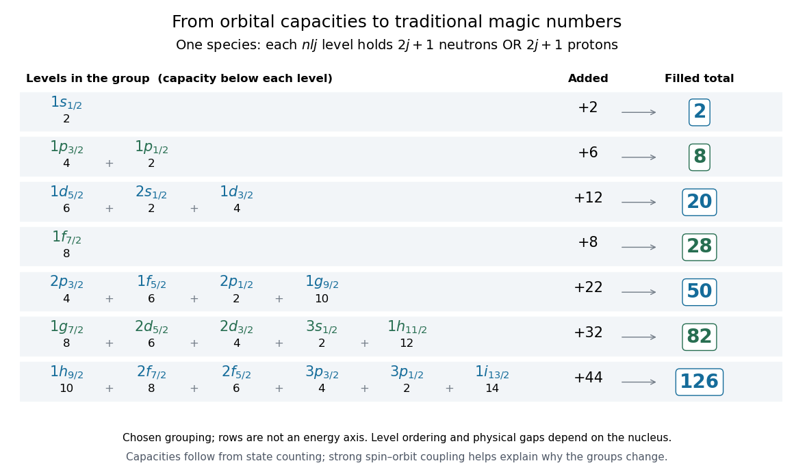
A proton number $Z$ or neutron number $N$ associated with a pronounced nuclear shell closure. The traditional sequence isThese count either species separately, rather than their sum $A=Z+N$. Calling a number magic summarizes a structural pattern; it does not promise that every isotope at that number is equally stable.

For example, in the chosen scheme the $20$-particle core plus the eight substates of $1f_{7/2}$ gives $28$. The next group contributes $4+6+2+10=22$, giving $50$. The following two groups contribute $8+6+4+2+12=32$ and $10+8+6+4+2+14=44$, giving $82$ and $126$. Counting verifies the capacities once the grouping has been chosen; it does not establish the physical energy gaps that justify that grouping.

Magnetic anisotropy can create a restoring torque that aligns a specimen in a magnetic field. For a small linearly responding object with uniaxial susceptibility difference $\Delta \chi$, volume $V$ and axis angle $\theta$ in an approximately uniform field, an orientation-dependent energy is $U=-V\Delta \chi B^2{\cos }^2\theta /(2{\mu }_0)$, up to an angle-independent term.

Positive $\Delta \chi$ favors alignment along the field; negative $\Delta \chi$ favors a perpendicular axis. Thermal angular fluctuations compete with this energy, so a preferred orientation becomes pronounced when the anisotropy scale exceeds $k_{B}T$. This induced-moment mechanism differs from the $-\mathbf{\mu }\cdot \mathbf{B}$ energy of a fixed permanent moment and is relevant to interpreting magnetic tweezers.