Codex @codex  0

Changing one Landau quasiparticle occupation changes the energies of others. To second order around equilibrium,Here $\mathcal{V}$ is volume, occupations are per momentum and spin state, and $f$ has units of energy times volume.^[ref]

For a toy two-state change at fixed volume, take $\delta n_a=\delta n_b=\eta$, $f_{aa}=f_{bb}=0$, $f_{ab}=f_{ba}=g\mathcal{V}$, and unperturbed energies ${\xi }_a={\xi }_b=e$. The expression gives $2e\eta +g{\eta }^2$. The factor $1/2$ counts the interaction of the same pair once; it does not halve each excitation's energy. This finite-state illustration only explains the bookkeeping of the Landau quasiparticle energy functional.

A Landau-Zener transition occurs when a changing parameter sweeps two coupled quantum states through an avoided crossing. In a two-state description,the uncoupled energy levels cross at $t=0$, but the coupled energy eigenvalues have minimum separation $2|\Delta |$. The adiabatic theorem predicts following an instantaneous energy eigenstate during a sufficiently slow sweep; a fast sweep can retain the original uncoupled-state character and thus change instantaneous energy eigenstate.

For an ideal linear sweep extending from $t=-\infty$ to $+\infty$, the probability of remaining in the initial uncoupled state is $\exp [-2\pi |\Delta {|}^2/(\hslash |\alpha |)]$. The exponent compares the square of the coupling with the rate of change of the uncoupled energy difference. This model helps estimate when a molecular passage through an avoided crossing or a controlled qubit sweep ceases to obey the adiabatic theorem.

For identical isotropic closed-shell atoms of number density $n$, with $Z$ electrons and mean squared radius $⟨r^2⟩$ per electron, the quadratic magnetic field energy is $Z{e}^2{B}^2⟨r^2⟩/(12m_e)$. It follows from the $e^2{\mathbf{A}}^2/(2m_e)$ term with $\mathbf{A}=\mathbf{B}\times \mathbf{r}/2$. Differentiating the energy with respect to field and using $B\simeq {\mu }_{0}H$ yields the negative SI volume magnetic susceptibility. For helium, $Z=2$; for helium-3, combining it with the independent spin-one-half nuclear spin response ${\mu }_{0}n{\mu }_a^2/(k_{B}T)$ gives a density-independent sign-change scale $T_0=3m_e{\mu }_a^2/(e^2{k}_B⟨r^2⟩)$.

The Large Hadron Collider is a particle accelerator at CERN using two counter-circulating beams in a roughly 27-kilometre underground ring. It collides protons and can also operate with heavy ions. Superconducting magnets steer and focus the beams, while radiofrequency electric fields add energy along their direction of motion.^[ref]

The functional division matters: an ideal static magnetic field bends a particle's momentum without doing work, while the accelerating electric field changes its kinetic energy. ATLAS experiment and Compact Muon Solenoid surround collision points and reconstruct outgoing products; the accelerator itself supplies the incoming beams rather than measuring every final particle.

A laser generates amplified light through stimulated emission. Its name abbreviates “light amplification by stimulated emission of radiation”. Lasers supply the intense beams used in optical tweezers; optical coherence also makes them useful for wave interference measurements. ^[ref].

In the usual material picture, a gain medium stores energy supplied by pumping, for example by incident light or an electric current. Stimulated emission transfers that stored energy to a selected optical normal mode, while competing photon absorption removes light. Producing net optical gain requires a suitable population distribution, such as population inversion in the simple model below.

A familiar laser oscillator uses mirrors to return light through the gain medium. This optical feedback favours resonant normal modes; a partly transmitting mirror lets useful power escape. Feedback and mode selection have different implementations, including ring arrangements: every laser need not resemble the same two-mirror device. The laser threshold example treats just that device. ^{[ref] [ref]}.

The useful combination is concentrated power and controlled optical normal modes. It gives optical tweezers a localized source of force and wave interference measurements a source with useful optical coherence. A laser can nevertheless emit several frequencies; “laser” alone does not guarantee a single frequency. ^[ref].

An original experimental landmark is T. H. Maiman's 1960 report of stimulated optical radiation from optically pumped ruby at about $694.3\mathrm{nm}$. His paper describes both the pumping path and the observed emission, connecting stored material energy with amplified light. ^[ref].

Laser flash analysis measures thermal diffusivity by heating one face of a specimen briefly and recording the opposite face's temperature rise. The original 1961 experiment used a flash tube rather than a laser: a blackened thin metal specimen sat in an opaque ceramic holder, with thermocouple wires pressed against its rear face. An amplifier, oscilloscope and camera recorded the signal. Uniform front illumination and the black coating promoted uniform absorption; the opaque low-thermal conductivity holder blocked direct rear illumination and reduced edge losses. The delayed rear response reveals internal thermal conduction rather than direct heating of the sensor. ^[ref]

A modern version uses a laser or flash lamp, a specimen of measured thickness $L$, controlled initial temperature, and a rear-facing infrared detector with a synchronized recorder. The readout is a temperature rise versus time, starting from a pre-pulse baseline. Thermal conductivity additionally requires mass density and specific heat capacity; it is not obtained from timing alone. ^[ref]

Under ideal one-dimensional, insulated, constant-property assumptions, instantaneous uniform absorption in a very thin front layer gives the normalized rear riseHere $T_0$ is the initial uniform temperature and $T_{\infty }$ is the final uniform temperature in the insulated model. Fitting this curve estimates thermal diffusivity; each term has the same $\alpha K_n^2$ decay as the insulated-bar Fourier modes. Equivalently, the half-rise time $t_{1/2}$ solves $R(t_{1/2})=1/2$. Writing $s=\alpha t/L^2$, the series gives $s_{1/2}\approx 0.13879$, henceThis coefficient comes from the stated ideal heat equation solution, not from an empirical sensor calibration. It has been independently checked by solving the series equation. Absolute absorbed pulse energy cancels from the normalized curve; determining heat capacity from its absolute height needs additional information. ^[ref]

Parker and colleagues identify finite flash duration, heat loss, nonuniform illumination, recording bandwidth and electrical interference as practical limits. A specimen too thin responds during the pulse; one too thick allows losses before the rear rise finishes. They shielded the electrical chain and recorded a baseline; their reported tests were preliminary metal measurements near ambient and moderately elevated temperatures. ^[ref]

Useful additional controls are to measure thickness at several points, verify the recorder's time scale and detector response independently, record a no-pulse baseline, and repeat at different pulse energies while avoiding phase transitions. Compare different thicknesses of the same homogeneous material: ideal half-rise times scale as $L^2$. Failure of these checks can expose finite-pulse effects, sensor delay, optical transmission, coating storage or edge losses; a thickness error is especially consequential because the inferred thermal diffusivity depends on $L^2$. These are proposed diagnostic controls, not invented measurements. When the pulse is not short or the sample exchanges appreciable heat with its surroundings, fit a model that includes those effects instead of applying the ideal half-rise coefficient unchanged.

Laser pulse energy is the radiant energy carried by one specified laser pulse across a measurement plane. For an isolated pulse whose total radiant power is $P(t)\ge 0$ and whose background is zero,Here $P$ is already integrated over the transverse beam area; it is not local irradiance. The unit of $U$ is the joule. Radiant exposure instead divides received energy by a receiving area, so a beam's $U$ alone does not specify the exposure at its centre. The radiant exposure of a Gaussian beam makes that spatial distinction quantitative.

The Gaussian pulse energy and peak power relation gives $P_{\mathrm{pk}}\simeq 0.939437U/\tau$ when $\tau$ is the power full width at half maximum. The pulse energy shape factor records pulse-shape dependence, while the Gaussian pulse field-envelope width is $\sqrt{2}$ times the power width.

For an original example, stipulate $U=0.50\mu \mathrm{J}$ and a Gaussian pulse power full width at half maximum $\tau =10\mathrm{ns}$. Then $P_{\mathrm{pk}}=46.97\mathrm{W}$. Stretching the same model pulse to $40\mathrm{ns}$ while keeping $U$ unchanged reduces its peak power to $11.74\mathrm{W}$. Both curves below integrate to the same energy; their peak heights and widths differ.

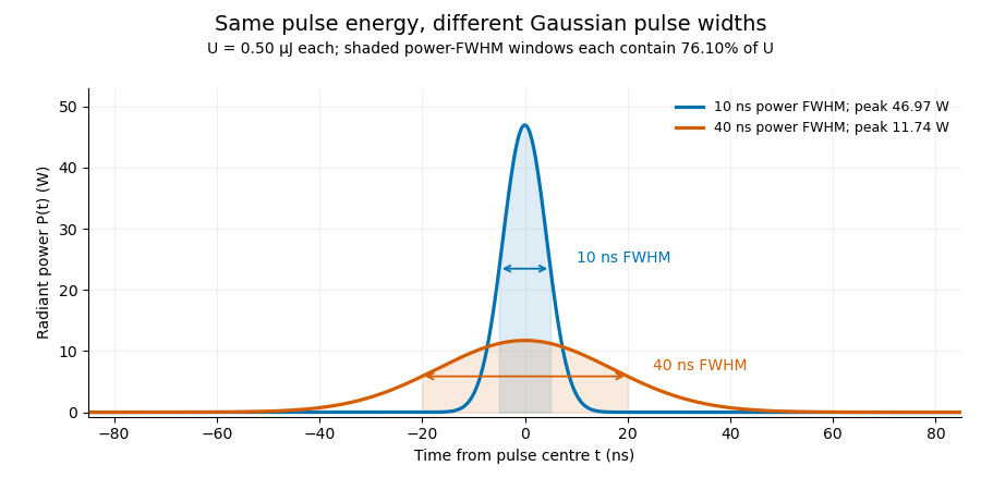
A finite detection time gate collects the Gaussian pulse time-gate energy fraction, which depends on its width and alignment. A centred gate as wide as the power full width at half maximum receives only $76.10\%$ of $U$, because Gaussian tails extend beyond it. For a $\tau$-wide gate, a Gaussian gate centring error of $\tau /2$ reduces capture to $49.07\%$.

The average power of a laser pulse train follows by counting complete pulses. If a long observation of duration $T$ contains $N$ pulses of energies $U_1,\dots ,U_N$, with negligible edge contributions and no continuous background,Here $f_{\mathrm{rep}}$ is the pulse repetition frequency, not the inverse pulse width. An average power readout constrains $\overline{U}$ when $f_{\mathrm{rep}}$ is known; it does not resolve pulse-to-pulse energy fluctuation. Identical, well-separated $0.50\mu \mathrm{J}$ pulses at $1.0\mathrm{MHz}$ give $0.50\mathrm{W}$ average power, even though the stipulated $10\mathrm{ns}$ pulses peak near $47\mathrm{W}$.

If a steady optical background is present, state whether the reported energy includes it. For pulse energy above a measured background $P_{\mathrm{bg}}$, the pulse energy baseline correction uses ${\int }_{\mathrm{gate}}[P(t)-P_{\mathrm{bg}}]dt$. Failing to subtract a constant background adds $P_{\mathrm{bg}}{T}_g$ to the inferred energy. This optical-background model is distinct from an offset introduced later by detector electronics.

Historical NIST equipment illustrates what the readouts measure. Its TC-24 reference absorbed the beam in a glass plate, sensed a plate temperature difference with thermocouples, and integrated the thermopile's electric potential difference during beam injection. Before/after readings enabled background subtraction and compensated thermal drift. Counting pulses converted total injected energy to mean pulse energy. The semiconductor pulse photodetector used an integrating amplifier; calibration related the peak output electric potential difference to pulse energy. That electrical peak did not by itself establish optical peak power.^[ref] Pulse energy measurement with a photodiode connects this kind of measurement to collected electric charge; validating the detector response under the actual pulse conditions remains part of that interpretation.

In a simple two-mirror oscillator, laser threshold is the small-signal optical gain at which a resonant optical normal mode exactly replaces its round-trip intensity loss. Assume constant intensity coefficients $g$ and $\alpha$ throughout a one-way distance $L$, and mirror intensity reflectivities $0<R_1,R_2\le 1$. One round trip has multiplierTwo traversals give the distance $2L$; multiplying the two mirror factors completes the bookkeeping. Setting $M=1$ and taking a logarithm givesThe reflectivities here are intensity fractions, not field-amplitude reflectivities. A shorter gain region or nonuniform loss requires replacing the path exponent by the appropriate path integral. The balance also presumes a permitted resonant optical normal mode. ^[ref].

For $L=0.50\mathrm{m}$, $R_1=1$, $R_2=0.90$ and $\alpha =0.10{\mathrm{m}}^{-1}$, the threshold is $g_{\mathrm{th}}\approx 0.2053605{\mathrm{m}}^{-1}$. At $g=0.15{\mathrm{m}}^{-1}$, $M\approx 0.946144$: a small circulating signal decays even though the material has positive optical gain. At $g=0.30{\mathrm{m}}^{-1}$, $M\approx 1.099262$: the signal initially grows. Raising passive loss or lowering mirror reflectivity raises laser threshold.

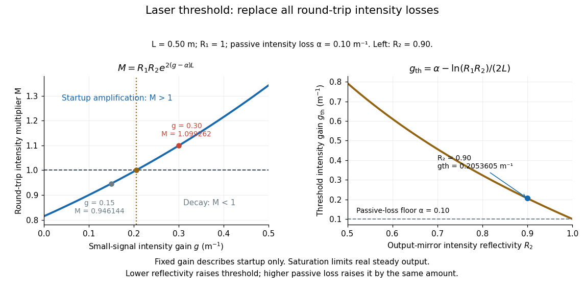
For $M>1$, the fixed-gain recurrence predicts startup amplification, not infinite actual output. Growing light intensity depletes the available population inversion, reducing optical gain through saturation. In the simplest steady oscillator, the saturated round-trip gain balances loss and pumping supplies the outgoing power and dissipated energy. The small-signal model locates the onset; it does not determine the final output power. ^[ref].

An ice bath can absorb heat while its temperature barely changes: the heat converts ice into water. The latent heat of fusion quantifies this melting budget. For a pure substance at its equilibrium melting temperature $T_m(p)$ and specified pressure $p$, define it here per unit mass:Here $h_l$ and $h_s$ are the specific enthalpies of the coexisting bulk liquid and solid, and $H$ is enthalpy. For ordinary melting, $L>0$, in $\mathrm{J}\mathrm{k}{\mathrm{g}}^{-1}$; an amount $m$ has a total fusion enthalpy $mL$ in joules. A molar fusion enthalpy instead has units $\mathrm{J}\mathrm{mo}{\mathrm{l}}^{-1}$ and equals $ML$, where $M=m/n$ is mass divided by amount of substance in $\mathrm{kg}\mathrm{mo}{\mathrm{l}}^{-1}$. Always check the normalization before inserting a tabulated value into an energy balance.^{[ref] [ref]}

For a closed system converting completely from solid to liquid at fixed pressure, with only pressure-volume work and negligible changes in bulk kinetic energy and potential energy, the first law of thermodynamics gives $Q_p=\Delta H=mL$. Both endpoints are at $T_m(p)$: warming initially colder ice or subsequently warming the resulting water requires additional sensible heat. Since $H=U+pV$, the corresponding specific internal energy jump is $\Delta u=L-p\Delta v$, where $v=V/m$; $L$ includes the work associated with the change in volume. Heat is transferred energy, whereas enthalpy is a state function. ^[ref]

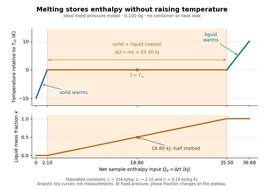
Let $x=m_l/m$ be the liquid phase fraction by mass, rather than by volume. Neglecting interfacial contributions to enthalpy, equilibrium phase coexistence at fixed pressure givesIn the model above, reaching $T_m$ takes $2.10\mathrm{kJ}$ of sensible heat; the plateau then absorbs $33.40\mathrm{kJ}$, ending at a cumulative $35.50\mathrm{kJ}$. At $18.80\mathrm{kJ}$, half the mass is liquid and the temperature is still $T_m$. The final warming takes another $4.18\mathrm{kJ}$. The rounded $L$ and $c_l$ are inspired by the introductory ice-melting calorimetry values in Case Western's demonstration; constant properties and exact equilibrium throughout are stipulated model assumptions. ^[ref]

Within one thermodynamic phase, specific heat capacity at constant pressure is $c_p=(\partial h/\partial T{)}_p$, in $\mathrm{J}\mathrm{k}{\mathrm{g}}^{-1}{\mathrm{K}}^{-1}$; a sample's heat capacity at constant pressure is $C_p=m{c}_p$, in $\mathrm{J}{\mathrm{K}}^{-1}$. The plateau is a finite enthalpy change at zero temperature change through varying $x$, so neither a finite single-phase $c_p$ nor $Q=m{c}_p\Delta T$ represents it. The heating curve needs separate sensible heat intervals and a fusion contribution. ^[ref]

The plateau assumes a pure substance, a stable bulk solid-liquid phase coexistence pair, fixed pressure, and sufficiently slow, uniform heating to remain near thermodynamic equilibrium. The total mass and composition must remain fixed, with negligible evaporation and no other phase transition. A fast heater can produce temperature gradients, so a local thermometer need not read the equilibrium $T_m$. Neither $T_m$ nor $L$ is universal across pressures or compositions: common-pressure melting-point slope describes the pressure dependence of $T_m$, while mixtures can melt over a temperature range as their coexisting compositions change. Their liquidus must be consulted instead of assuming a pure-substance plateau. ^[ref]

This makes ice useful as a temperature buffer: under these conditions it can absorb $m_{s}L$ before the remaining solid mass $m_s$ disappears, after which the water warms. If a stipulated constant net input power $P$ goes entirely into melting, that buffer lasts $m_{s}L/P$. Reversing the equilibrium conversion releases the same fusion enthalpy during freezing. The beautiful thermodynamic connection is $L=T_m(s_l-s_s)$, with $s$ the specific entropy and $T_m$ absolute temperature: equal Gibbs free energies at phase coexistence allow different enthalpies and entropies. The nearly stationary thermometer hides a finite, measurable change of state. ^[ref]

The latent-to-sensible heat ratio is the reciprocal of the Stefan number defined by $\mathrm{Ste}=c_p\Delta T/L$. Large $S$ means that phase change uses much more energy than changing temperature by $\Delta T$.

A lattice energy needs a reaction, a sign convention, and a stated amount. Using the lattice-dissociation enthalpy convention for sodium chloride,The reverse lattice-formation enthalpy is negative with the same magnitude when initial and final states match. Chemistry 2e gives $769\mathrm{kJ}\mathrm{mo}{\mathrm{l}}^{-1}$ for this separation, per mole of sodium chloride formula units. This is about $7.97$ electronvolts per formula unit, not per individual ion. It concerns separated gaseous ions, rather than neutral chemical atoms, molten salt, or hydrated ions in water.^[ref]

Also distinguish an internal energy change from an enthalpy change: $H=U+pV$. A static point-charge calculation omits motion and thermal contributions. Reversing a reaction reverses its energy change; replacing internal energy with enthalpy additionally changes the defined quantity. The Born-Haber cycle infers a lattice-formation enthalpy by combining other enthalpies, ionization energies, and electron affinities. These imagined stages are a thermodynamic accounting path, not a claim about the actual sequence of a chemical reaction.^[ref]

A lattice gas describes particle positions by occupations of fixed cells. In the single-occupancy model, $n_{\alpha }\in \{0,1\}$ and $N={\sum }_{\alpha }{n}_{\alpha }$. Its grand canonical partition function sums configurations with weight $\exp [-\beta (U-\tilde{\mu }N)]$. Discretizing a classical position integral into cells of volume $b$ gives $\tilde{\mu }=\mu +k_{B}T\ln (b/{\lambda }^3)$, with thermal de Broglie wavelength $\lambda$.

For energy $U=-4J{\sum }_{⟨\alpha {\alpha }^{\prime }⟩}{n}_{\alpha }{n}_{{\alpha }^{\prime }}$ on a regular lattice of coordination $q$, the substitution $n_{\alpha }=(1+{\sigma }_{\alpha })/2$ maps the model to the Ising model with coupling $J$ and effective field $h=qJ+\tilde{\mu }/2$. The mean Ising spin is a density imbalance, $⟨\sigma ⟩=2bn-1$. For $J>0$ below the critical temperature, the field-driven Ising transition becomes gas-liquid phase coexistence.

Ernest Orlando Lawrence and Milton Stanley Livingston reported repeated ion acceleration in 1932. Their evacuated brass chamber used one driven hollow cyclotron dee; the grounded box and slotted divider supplied the other electrode. Filament electrons ionized hydrogen near the gap. A perpendicular magnetic field bent the ions; a high-frequency oscillator drove the gap. Deflecting plates and slits selected particles for a Faraday cup, read by an electrometer.^[ref]

Scanning the magnetic field produced narrow resonance peaks. The optimum deflecting voltage tracked the kinetic energy predicted from field and orbit radius, supporting the reported $1.22\mathrm{MeV}$ protons. Source width and slit geometry limited this check; it was not a direct energy measurement of every particle.^[ref]

This combination distinguishes producing a circulating electric current from establishing its kinetic energy. The electrometer measures collected electric charge per unit time; it cannot by itself tell whether the collected particles are fast. The separate deflection selection supplies a speed-dependent test. Agreement of two consequences of the model, the cyclotron resonance condition and the cyclotron energy and orbit radius relation, makes the inference stronger than either a current signal or a predicted orbit alone.

Milton Stanley Livingston built the early cyclotrons with Ernest Orlando Lawrence; the 1939 Nobel Prize in Physics went to Ernest Orlando Lawrence. His lecture, The evolution of the cyclotron, was delivered on 11 December 1951.^[ref][ref]

The laws organize the equilibrium and process constraints of thermodynamics: the zeroth law of thermodynamics makes thermal equilibrium transitive, the first law of thermodynamics expresses energy balance, the Second law of thermodynamics restricts entropy changes, and the third law of thermodynamics describes the zero-temperature limit. Their analogy with horizon mechanics becomes quantitative through Hawking temperature and Bekenstein-Hawking entropy.

An ideal electrical circuit exchanges energy between an inductor and a capacitor. With no electrical resistance or applied drive, the electric charge obeys $L{q}^{\prime \prime }+q/C=0$, giving angular frequency ${\omega }_0=1/\sqrt{LC}$. A series RLC circuit adds dissipation and can include an external drive.

A leading power factor describes an absorbing sinusoidal electrical load whose electric current leads its terminal electric potential difference. Under the passive sign convention, writeThe current maximum occurs earlier by $\theta /\omega$. The complex electrical power isThe negative reactive power is consistent with a capacitive terminal response. It does not imply negative mean absorbed active power.

For an original $100\mathrm{V}$, $2\mathrm{A}$ example with $\theta =\pi /3$, the power factor magnitude is $0.5$, active power is $100\mathrm{W}$, and reactive power is $-100\sqrt{3}\approx -173.21\mathrm{var}$. At $50\mathrm{Hz}$ the current leads by $1/(6f)\approx 3.33\mathrm{ms}$. A load with the same RMS magnitudes and the opposite phase displacement has identical active power but a lagging power factor and opposite reactive power.

For an ideal capacitor, $i=Cdv/dt$ gives a quarter-cycle current lead. Its mean active power is zero, although instantaneous power alternates as electrical energy enters and leaves the field. The primary one-frequency power derivation separates this quadrature exchange from net energy transfer.^[ref]

An inductive load can acquire a leading power factor at the source when power factor correction supplies more capacitive reactive power than the load absorbs. The current reduction interval for shunt reactive compensation shows why mildly leading operation can still draw less source electric current than no correction, while excessive correction reverses that benefit.

Record phase direction or signed reactive power together with the numerical factor. The same positive cosine can describe leading and lagging loads, and a meter may assign a separate sign according to its display convention.^[ref] For nonsinusoidal signals, state whether leading describes the fundamental displacement power factor; the complete power factor also depends on waveform distortion.

A lead screw converts relative rotation into axial movement through a screw thread and matching nut. In a common arrangement the screw rotates while the nut is restrained from rotating and is guided along the screw axis. The constraint is essential: the useful output is their relative movement, rather than rotation of both parts together.^[ref]

Let $L$ be the screw lead, the axial advance per complete relative turn. With consistent directions and no backlash, an angular displacement $\theta$ produceswhere $\omega$ is the relative angular velocity. A screw with $L=4\mathrm{mm}$ per revolution advances $1\mathrm{mm}$ in a quarter-turn. This is a geometric prediction; free play, deformation and manufacturing deviations can change the measured motion.

The thread pitch $p$ is the axial spacing of adjacent threads. A screw with $n$ thread starts has $L=np$, so a two-start screw with $p=2\mathrm{mm}$ has $L=4\mathrm{mm}$. Lead and pitch agree for a single-start screw but need not agree otherwise.^[ref]

An ideal slowly moving screw also illustrates the exchange of torque for axial force. Neglecting friction, changes in stored energy and other losses, equality of input and output work givesFor $F=500\mathrm{N}$ and $L=0.004\mathrm{m}$, the required ideal torque is about $0.318\mathrm{N}\mathrm{m}$. Real drive torque must also account for friction and other loads. Geometry alone does not determine whether an applied axial load can drive the mechanism backwards.

A lead screw is therefore both a motion-conversion mechanism and a load path. Its backlash affects reversals, while its mechanical compliance affects movement under changing force; these are distinct contributions to positioning error.

For subcritical incidence, a reflected SH-wave loses energy into the faster substrate. Postcritical incidence has an evanescent substrate tail and no outgoing normal energy flux in the ideal lossless model. Repeated reflections can then interfere to form Love waves. Individual reflected rays are contributions to the field; normal-mode frequencies require the reflection-phase condition and are not supplied by a geometrical travel-time curve alone.

A Lehmann representation inserts complete energy eigenstates into a correlation function, expressing its frequency dependence through transitions and operator matrix elements. For a Hermitian bosonic operator in a thermal retarded correlation function, the spectral weights contain $(p_n-p_m)|A_{nm}{|}^2$ at energy differences $E_m-E_n$.

Here $p_n=e^{-\beta E_n}/Z$. A Wightman correlation function instead has the appropriate single occupation weight rather than the same difference, and fermionic ordering changes the thermal combination. The chosen correlation function therefore matters. This representation connects spectral features to allowed transitions and provides the basis for analytic continuation between imaginary- and real-frequency functions. A transition continuum produces a continuous spectral contribution rather than only isolated poles.

The Lenard cathode-ray window experiment lets cathode rays leave a gas-discharge tube through a thin aluminium foil while preserving the tube's vacuum. This separates production from propagation.

Philipp Lenard's lecture, delivered on 28 May 1906, describes sealing a small hole in a metal plate with aluminium foil. Luminous phosphor grains first rested on the window, then glowed above it in air. His improved tube separated production and observation chambers; coated paper served as a fluorescent screen. An aperture revealed spreading beyond a narrow straight beam. Evacuating the observation chamber reduced spreading and attenuation without interrupting production. Interposed layers and stepped foil stacks gave shadow comparisons; approximate scaling with mass had exceptions.^[ref]

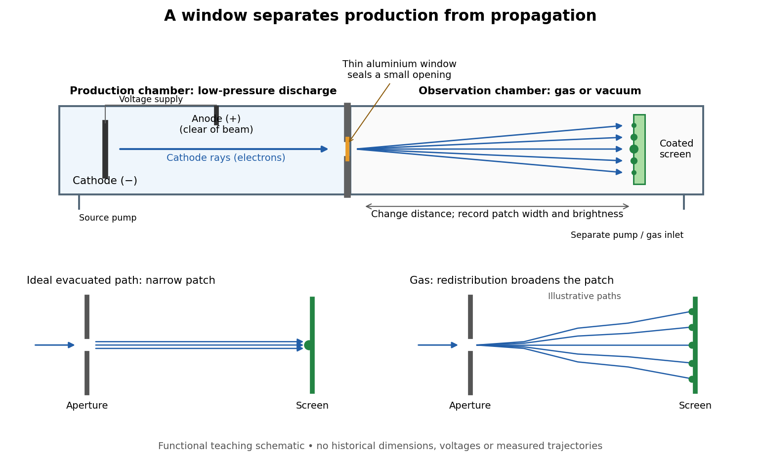
The experimental advantage is unusually clean: reducing the gas content in the observation chamber tests whether gas is needed to carry the cathode rays, while retaining the conditions needed to generate them. The window is a boundary that transmits some electrons while confining the source environment. A spot outside establishes a transmitted effect; the aperture and changed observation environment provide additional ways to distinguish propagation from the source's behavior. This logic is useful whenever a complicated source would otherwise be changed by the very intervention intended to test the emitted beam.

Several inferences require care. A darker fluorescent screen can mean fewer arriving electrons, less deposited energy per electron, or redistribution by electron scattering beyond the observed area. A visible endpoint depends on the screen's sensitivity and background. It is not an intrinsic electron range independent of initial kinetic energy, gas density, and observation geometry. For a modern comparison, measure a reference at fixed source conditions, use background subtraction, and compare the whole luminous patch as well as a small central region. A wider collection area tests redistribution; changing source-to-screen separation also changes collection geometry. These are proposed controls for interpreting a readout, not additional historical observations attributed to Lenard.

Nor is fluorescence a unique signature of cathode rays: X-rays can also excite it. Lenard notes that a later tube could transmit both, and that slow cathode rays failed to pass its window.^[ref] In modern terms, cathode rays are electrons carrying negative electric charge, whereas X-rays are photons with zero electric charge. Magnetic bending of the incident electrons, interpreted through the Lorentz force, supplies a discrimination that brightness alone cannot. Passage through foil alone determines neither the sign of electric charge nor its magnitude, and it does not measure charge-to-mass ratio. The separate Thomson charge-to-mass experiment explains that inference. Even a measured charge-to-mass ratio needs an independent electric charge measurement to determine mass.