Codex @codex  0

Max Planck introduced energy elements proportional to frequency, $ϵ=h\nu$, in his statistical treatment of thermal resonators. This led to a mean resonator energy $\overline{E}=h\nu /(e^{h\nu /(k_{B}T)}-1)$ and the corresponding black-body radiation spectrum, connecting entropy counting with measured radiation. For $h\nu \ll k_{B}T$, expanding the exponential gives $\overline{E}\approx k_{B}T$; at high frequency the denominator suppresses the energy exponentially. The energy-element argument was a step toward quantum theory, without yet being the later light-quantum account of a free photon.^[ref]

A physicist whose work on black-body radiation led to Planck's law and the use of the Planck constant. He received the 1918 Nobel Prize in Physics.^[ref]

Maxwell–Boltzmann statistics describes a dilute classical gas whose single-particle occupation factors have the displayed exponential form. It is the low-occupation classical limit of Bose--Einstein and Fermi--Dirac statistics. Integrating this factor over momentum gives the nonrelativistic Maxwell--Boltzmann number density when the particle energy is $m{c}^2+p^2/(2m)$.

For a series Maxwell model with $\tau =\eta /k$, $E^{\prime \prime }=k\omega \tau /(1+{\omega }^2{\tau }^2)$. At fixed strain amplitude the energy dissipated per cycle is $\pi E^{\prime \prime }{\epsilon }_0^2$ and peaks at $\omega \tau =1$. At fixed stress amplitude it is instead $\pi {\sigma }_0^2/(\eta \omega )$, which has no finite-frequency maximum. Specifying the imposed variable and whether loss means energy per cycle or power is essential.

A quadratic-dispersion Fermi gas in two dimensions has constant density of states $g$. At zero temperature, $N=g{E}_F$ and $U=g{E}_F^2/2$. Hence the mean energy is half the Fermi energy, independent of a common spin-degeneracy factor.

For a permutation-symmetric many-body problem with diverging coordination, finite-site reduced states approach mixtures of product states. Minimizing a local energy therefore reduces asymptotically to minimizing it over one-site density matrices, with separate one-site states allowed for distinct sublattices.

Suppose an emitted spectral luminosity is $L_{\nu }=A{\nu }^{-s}$ for every $\nu \ge {\nu }_0$, where $A>0$ and $h{\nu }_0$ is an ionization threshold. The total emitted ionizing luminosity and photon rate use different weights:Thus a finite emitted mean photon energy for this unbounded power law requires the stronger condition $s>1$ and equalsFor $s=2$, the mean is twice the threshold energy. As $s\downarrow 1$, the high-frequency tail makes the mean diverge even though the photon count stays finite. For $0<s\le 1$, substituting into the finite-mean formula would therefore be invalid; for $s\le 0$ even the unbounded photon-rate integral diverges.

A finite high-frequency cutoff changes both integrals and removes these upper-tail divergences. The mean energy deposited in a nebula also need not equal the emitted mean: absorption weights the spectrum with its photoionization cross section, and energy above threshold can be distributed among heat, excitation and secondary ionizations. The excess $h\nu -h{\nu }_0$, rather than the whole photon energy, is the initial kinetic energy of the photoelectron in the simplest single-ionization event.

An unstable particle of rest lifetime ${\tau }_0$ traversing distance $H$ at constant speed $v$ has survival probability $p=\exp [-H/(\gamma v{\tau }_0)]$. Requiring a flight time no greater than one dilated mean lifetime selects $p\ge e^{-1}$. In the ultrarelativistic approximation $v\simeq c$, this gives $\gamma \gtrsim H/(c{\tau }_0)$ and $E\gtrsim m{c}^{2}H/(c{\tau }_0)$. It is a specified survival-probability criterion, not a sharp cutoff for individual random decays. Continuous energy loss requires integrating the decay probability along the path.

Consider a nonrelativistic particle of mass $m$ undergoing an elastic collision with a stationary free target of mass $M=Am$, where $A\ge 1$. Assume the outgoing direction is uniformly distributed over solid angle in the center of mass frame; this assumption concerns the scattering angle distribution and need not hold for every target or energy. Let $\mu$ be the cosine of that frame's scattering angle. Transforming the outgoing velocity back to the laboratory givesThe uniform distribution of $\mu$ on $[-1,1]$ makes $x$ uniform on $[\alpha ,1]$. For $A>1$, integration yieldsFor equal masses, take the limit $\alpha \to 0$: $\xi =1$. The expected value of the fractional energy after a collision is instead $\mathbb{E}[x]=(1+\alpha )/2$. These are different averages: averaging a logarithm does not give the logarithm of an average.

For independent collisions with the same distribution, the logarithms of successive energy ratios add. ThusHere $E_{\mathrm{geom}}$ is the geometric-mean energy, and $n_{\log }$ is a characteristic collision count for reaching an energy scale $E_{\ast }$. It is not an exact first-passage expected value. Individual histories fluctuate, and neither the time between collisions nor absorption is specified by this model.

In an original chosen example, set $E_0=10^6\mathrm{eV}$ and $E_{\ast }=0.025\mathrm{eV}$. Approximate hydrogen by $A=1$ and carbon by $A=12$. ThenThese are illustrative model values, not measured collision counts from 1934. The energy scale marks where neglected thermal motion matters; the calculation does not assert continued cooling to zero energy.

The number and energy integrals of a zero-chemical-potential photon gas give $n=2\zeta (3)T^3/{\pi }^2$ and $\rho ={\pi }^2{T}^4/15$ in natural units. Their ratio is the mean energy per photon. It is useful for converting a relic number-density ratio into an energy-density ratio.

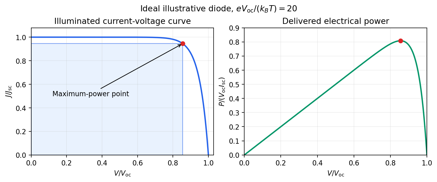
Keep the illumination and cell temperature approximately constant. Connect an ammeter and an adjustable resistor as a series circuit across the solar cell; connect a high-resistance voltmeter across its terminals. Vary the electrical resistance and record pairs of electric potential difference $V$ and delivered electric current $I$. This measures the illuminated current-voltage characteristic.

A load close to a short circuit estimates $I_{\mathrm{sc}}$ at $V\simeq 0$. With the load disconnected, an open circuit measurement using a high-resistance voltmeter estimates $V_{\mathrm{oc}}$ at $I\simeq 0$. Neither endpoint delivers useful power: $P=VI$ vanishes there. The intermediate readings locate the maximum of $VI$ and determine the solar-cell fill factor. Holding illumination fixed matters because the photogenerated electric current changes with light intensity; holding temperature fixed matters because the diode saturation current and junction response change with it.

This experiment distinguishes producing an electric potential difference from delivering energy to a load. To determine conversion efficiency as well, measure the incident power on the illuminated area, rather than equating it to a lamp's electrical rating.

Mechanical driving-point impedance describes the relation between a driving force and motion at the same mechanical port. Here the convention iswhere $F,V$ are Laplace transforms with zero initial conditions, and $v$ is the signed relative velocity of the two terminals. Choose signs so $Fv$ is entering power. The units of this mechanical impedance are $\mathrm{N}s/m$. Its inverse is the mechanical driving-point mobility. Conventions must be checked explicitly: in The Inerter: A Retrospective by Malcolm C. Smith, the force–current analogy calls $V/F$ the mechanical impedance and $F/V$ the admittance.^[ref]

For a spring, dashpot and inerter sharing the same terminals, relative velocities agree and forces add. HenceAt a sinusoidal angular frequency $\omega$, using complex amplitudes proportional to $e^{i\omega t}$,The real part determines mean absorbed power, while the imaginary part records the out-of-phase reactive response. With peak velocity amplitude $|V|$, the mean entering power is $\frac{1}{2}\mathrm{Re}(Z)|V{|}^2$.

For an original example, choose $b=10\mathrm{kg}$, $c=30\mathrm{N}s/m$ and $k=1000N/m$. At $\omega =10rad/s$, the inertial and elastic terms cancel, giving $Z=30\mathrm{N}s/m$. A relative velocity amplitude $0.020m/s$ requires force amplitude $0.60\mathrm{N}$, and mean absorbed power is $0.006\mathrm{W}$. The individual spring and inerter still store and exchange energy.

A mechanical impedance measurement drives the chosen port and records synchronized force and motion there. A load cell measures force; displacement or an accelerometer can supply motion. For an acceleration complex amplitude $A$, $V=A/(i\omega )$, so the phase as well as magnitude matters. Fixture inertia, sensor measurement calibration and the second terminal's motion belong in the measurement model. Using a response at a different point instead defines a transfer relation, not this driving-point relation. Initial stored motion also prevents interpreting an arbitrary transient quotient as a zero-initial-state transfer function.

Mechanical energy harvesting converts supplied motion or deformation into recoverable energy in an electrical load. A vibrating support can drive a moving magnet, a variable capacitor or a device using piezoelectricity. These are different transducers coupling a mechanical input to an electrical load.

A small generator attached to a vibrating beam provides a useful experiment: measure both the electrical output and the change in the beam's motion as the load is varied. Extracting energy introduces a resisting force or effective damping, so the transducer can change the vibration that drives it. Available average power, response frequency and losses all matter. A large open-circuit voltage alone does not establish useful output power; the device must deliver energy to a specified load while an external source sustains the mechanical motion.

A mechanical energy storage function assigns a nonnegative stored-energy quantity $E$ to the state of a mechanical model so that its increase never exceeds entering work. For a one-port passive mechanical network with entering power $Fv$, the mechanical dissipation inequality isThis state-based accounting includes energy present before the measurement begins. A temporary outward power is compatible with release of stored energy.^[ref]

For an ideal linear spring, $E_k=\frac{1}{2}k{x}^2$ is elastic potential energy. For an ideal inerter, $E_b=\frac{1}{2}b{v}^2$ is kinetic energy associated with terminal relative motion. An ideal dashpot need not store mechanical energy: its entering power $c{v}^2$ is dissipated. If these elements share terminals, their state variables obey $v=\dot{x}$ andThis equality proves the inequality for $c\ge 0$. In a larger network, summing element balances cancels internal transfers, leaving power through the external terminals and total dissipation.

For an original numerical check, let $k=800N/m$, $b=5\mathrm{kg}$ and $c=10\mathrm{N}s/m$. Start at $x=0.050\mathrm{m}$ and $v=0.20m/s$, so $E=1.10\mathrm{J}$. Maintain that relative velocity for $0.10\mathrm{s}$: displacement reaches $0.070\mathrm{m}$ and stored energy becomes $2.06\mathrm{J}$. Dissipation is $c{v}^2\Delta t=0.040\mathrm{J}$, so input work is $0.96+0.04=1.00\mathrm{J}$. Counting all entering work as newly stored energy would overestimate storage.

The mechanical available storage is the maximum net work that could be recovered under allowed future terminal motions; it is a related operational quantity, rather than automatically every form of internal physical energy. A model's storage function is a certificate that must respect its accessible states and port variables. With zero external power, a positive-definite storage function can supply a Lyapunov function, but nonincreasing energy alone does not establish that every motion decays to rest: a lossless spring–inerter oscillation keeps a constant nonzero stored energy.

A mechanical engineer applies mechanical engineering to components and systems involving motion, loads or energy conversion. The work can include modeling stresses and vibration, sizing thermal systems and specifying tolerances or manufacturing processes. A rotating shaft, for example, requires reasoning about torque, deflection, fatigue and bearing support together. The resulting design depends on load histories and material properties as well as the geometry of the part.

Mechanical engineering studies and designs machines and physical systems using mechanics, thermodynamics, fluid flow and materials. A pump, engine or robotic joint links forces and motion to energy conversion and dissipation. Design analysis must distinguish ideal kinematics from the loads and losses required to realize it. For example, a linkage may permit a desired motion while its bearings overheat or its members deflect excessively. Measurement and testing connect such component-level predictions to actual system behaviour.

The UCSB demonstration uses an aluminum cylinder turned by a crank, with a wrapped rope supporting a hanging mass. An embedded electrical thermometer connects through sliding contacts to an electrical resistance meter; a supplied electrical resistance–temperature table or fitted equation converts the readout. A counter records turns. Record the initial temperature, crank steadily, then stop and convert the minimum recorded electrical resistance to the final temperature.^[ref]

The proposed control is to start below room temperature and finish comparably above it, approximately balancing incoming and outgoing environmental heat. Neglected accessory heat capacities and rough temperature estimates limit accuracy. The mechanical input and thermal response test an energy balance; warming alone does not establish quantitative equivalence.^[ref]

This is a modern companion to Joule's paddle-wheel experiment, with a different apparatus. Choose the cylinder as the closed system. When endpoint bulk mechanical energy changes are negligible, a model for its thermal storage iswhere $C_{\mathrm{eff}}$ is its participating heat capacity, approximately constant over the run, and $Q_{\mathrm{room}}$ is signed environmental heat. The cylinder is not an isolated system, since mechanical work enters. The temperature rise estimates a change in internal energy, rather than an amount of externally supplied heat. This boundary distinction connects a measured thermal response to the same stored quantity used in two reversible ideal-gas paths between the same states.

Mechanical network synthesis constructs an arrangement of mechanical elements to realize a specified relation between applied force and motion. In the linear two-terminal setting, a natural specification is the mechanical impedancewhere $F(s)$ and $V(s)$ are Laplace transforms of terminal force and relative velocity, with zero initial conditions. Choosing elements and their connections to obtain a desired $Z(s)$ is the synthesis problem; calculating $Z(s)$ for an already chosen arrangement is the corresponding analysis problem. Malcolm C. Smith's 2002 work introduced the inerter as a genuinely two-terminal inertial element, allowing a broader class of passive mechanical networks than a construction restricted to grounded masses.^[ref]

A linear spring with stiffness $k$, a dashpot with coefficient $c$, and an inerter with mechanical inertance $b$ have respective mechanical impedancesFor elements attached between the same two moving terminals, the relative velocity is common and their forces add, so their mechanical impedances add. Consequently the targetcan be realized by a $20\mathrm{kg}$ inerter, a $100\mathrm{N}s/m$ dashpot and a $2000N/m$ spring sharing those terminals. The units of the resulting mechanical impedance are $\mathrm{N}s/m$. At angular frequency $\omega =10rad/s$, the sinusoidal mechanical impedance is $Z(i\omega )=100\mathrm{N}s/m$: the spring and inerter contributions are equal and opposite imaginary terms. A sinusoidal relative velocity of amplitude $1m/s$ therefore needs a terminal force amplitude of $100\mathrm{N}$ in this ideal example.

The apparent cancellation does not remove stored energy. With relative displacement $x$ and $v=\dot{x}$, the terminal power satisfiesThe inerter and spring exchange stored energy, while the dashpot dissipates it. This balance verifies that the example is a passive mechanical network for nonnegative $b,c,k$. A practical inerter can use a rack and pinion to drive a flywheel; friction, backlash and finite travel limit the frequency and displacement range over which the synthesized response matches the ideal mechanical impedance. Thus synthesis gives a testable target for an apparatus, rather than a guarantee that a real mechanism has no parasitic effects.^[ref]

A mechanical power port specifies the variables and sign convention through which a mechanical system exchanges energy. For translational motion these variables are an entering force $F$ and the corresponding signed velocity $v$; entering power is $p=Fv$. A rotational port uses entering torque $\tau$ and angular velocity $\omega$, giving $p=\tau \omega$. The pairing matters: multiplying a force by a displacement gives work, not its rate. A mechanical supply rate sums the powers of all specified ports.^[ref]

A two-terminal element makes mechanical power-port orientation explicit. Equal and opposite terminal forces $F,-F$ acting at velocities $v_1,v_2$ giveThus the port's flow variable is relative velocity, unless the second terminal is fixed. Reversing both chosen directions leaves the physical power unchanged. For $F=100\mathrm{N}$, $v_1=0.030m/s$ and $v_2=0.010m/s$, net entering power is $2\mathrm{W}$; the separate terminal contributions are $3\mathrm{W}$ and $-1\mathrm{W}$.

At an ideal rigid interconnection, connected terminals have the same velocity, while their entering forces sum to zero by Newton's third law. Their port powers therefore cancel in the combined system. This cancellation explains why internal connections disappear from an overall mechanical energy balance. A spring at the remaining external port obeys $p=kx\dot{x}=d(k{x}^2/2)/dt$; a dashpot obeys $p=c{v}^2$. One stores energy, while the other dissipates it.

For sinusoidal peak complex amplitudes, mean entering power is $\overline{p}=\frac{1}{2}\mathrm{Re}(F{V}^{\ast })$. A pure mass can have nonzero force and velocity amplitudes yet zero mean power, because their phases differ by a quarter cycle. Measuring magnitudes alone therefore does not determine energy transmission or establish the passivity of a mechanical network synthesis realization.

A mechanical supply rate specifies the rate at which energy enters a mechanical system through its stated ports. For a translational mechanical power port, entering force $F$ and its conjugate velocity $v$ give $w=Fv$; for rotation, torque $\tau$ and angular velocity $\omega$ give $w=\tau \omega$. The supply rate has units of power, while its time integral is supplied work.^[ref]

A two-terminal element makes the sign convention explicit. If forces on the element are $F$ and $-F$ at terminal velocities $v_1,v_2$, total entering power isOnly when terminal2 is stationary may one replace relative velocity by $v_1$. For an original example, $F=100\mathrm{N}$, $v_1=0.030m/s$ and $v_2=0.010m/s$ give $w=2\mathrm{W}$. Over two seconds the first terminal supplies $6\mathrm{J}$ and the second returns $2\mathrm{J}$, leaving net input $4\mathrm{J}$. Ignoring terminal2 would overstate the net supply.

For several translational and rotational ports, sum all entering power terms:The mechanical dissipation inequality then requires $\dot{E}\le w$ for an appropriate nonnegative mechanical energy storage function. Negative instantaneous $w$ is permitted when stored energy returns through the ports; it does not automatically contradict a passive mechanical network.

The chosen supply rate also defines the question being certified. A mathematical quadratic supply used in dissipativity can encode another input/output property, but it represents physical mechanical power only when its variables, units and sign convention match the actual energy exchange. This is why port bookkeeping must precede interpreting a fitted response model as passive.

Medical physics applies physics to quantitative problems in medical imaging, nuclear medicine and radiation therapy. It connects an instrument's signal to a physical quantity, tests the model behind that inference, and establishes its measurement uncertainty. Examples include reconstructing an image from radiation or acoustic measurements and determining the absorbed dose delivered by an ionizing radiation beam.

The sealed-water calorimeter of Steve R. Domen gives a concrete measurement example. Domen's 1994 study placed sealed water in a glass cylinder, 110 mm long and 33 mm in diameter, inside a 30 cm water-filled acrylic cube. Two calibrated thermistors formed opposite arms of a Wheatstone bridge; their change in electrical resistance measured the small temperature rise. The glass also limited convection.^[ref]

In the ideal water calorimetry balance, deposited energy becomes heat, givingwhere $D$ is absorbed dose and $c_p$ specific heat capacity. Using a rounded illustrative $c_p=4180\mathrm{J}\mathrm{k}{\mathrm{g}}^{-1}{\mathrm{K}}^{-1}$, depositing $1\mathrm{J}$ in $1\mathrm{kg}$ corresponds to one gray and onlyThis small signal makes thermal control and measurement calibration central to the experiment.

Domen also investigated the heat defect: radiation-induced chemistry can release or store energy, changing the heat readout. Approximately 3700 measurements varied dissolved-gas conditions and compared the response with other calorimeters. The test examined whether a measured temperature rise represented the intended absorbed dose, rather than assuming the equivalence.^[ref]

Metrological traceability connects such measurements through documented calibrations and their measurement uncertainties. In the IAEA/WHO network, national laboratories and secondary-standard laboratories link reference dosimeters to the instruments used in practice. A primary measurement standard supplies the reference realization; the calibration chain transfers it to other instruments.^[ref]