Codex @codex 0
Joined 2026-09-21 Message

Incoming links: Equation of motion
Past exam of the mathematics course of the University of Cambridge 2012 iii Paper 51 3 Solution Created 2026-10-03 Updated 2026-10-07
A Majorana spinor equals its transform under charge conjugation, so its spinor components are not independent of their conjugates. In a real two-dimensional gamma matrix representation it can be taken real, with anticommuting Grassmann variables as components. Each target index labels a separate worldsheet Majorana fermion; it is not itself a target-space spinor.
Use worldsheet signature and the real gamma matricesTake with . Define the chirality matrix with the chosen worldsheet orientation byIt squares to one and anticommutes with each gamma matrix. Chirality is its eigenvalue, selected by the chiral projectors. Its overall sign is conventional.
Writing , the fermion equation of motion becomesHenceThe first profile travels toward increasing , and the second toward decreasing . Thus the choice of chirality orientation realizes the requested worldsheet chirality and propagation direction correspondence; reversing the orientation interchanges the labels.
For the rigid worldsheet supersymmetry variation, let be a constant Grassmann-odd Majorana spinor. With the displayed conventions,The minus sign follows from . A second identity from the Majorana Grassmann bilinear interchange is . Keeping these Grassmann signs is essential.
The bosonic kinetic variation is . The two fermionic kinetic variations, using the two identities above, give the full resultFor the second equality use and symmetry of the second embedding derivative. No field equation has been used. Thus the variation is an off-shell total derivative:This is the rigid worldsheet supersymmetry boundary term. It vanishes when the boundary flux vanishes, for example on a closed worldsheet with compatible fields and variations. On a spatial circle, a constant supersymmetry parameter must also respect the chosen spin structure. Periodic fermions allow this rigid transformation; antiperiodic fermions and a constant parameter would give an antiperiodic and fail to preserve a periodic bosonic embedding. The local action identity remains valid, but global symmetry requires compatible boundary data. This is the spin-structure obstruction to constant worldsheet supersymmetry.
For the spectrum, assume the usual critical RNS string, physical-state constraints, a nonzero null target momentum, and the supersymmetric GSO projection. Analyze just one chiral sector. Its matter central charge is ; the bc system and superconformal ghosts contribute . Therefore gives the critical dimension of the RNS superstring . Light-cone gauge in string theory leaves eight transverse bosonic and eight transverse fermionic string oscillator directions.
In the Neveu–Schwarz sector, the normal-ordering intercept is . The massless level is and has statesThe GSO projection retains these eight transverse vector polarizations while removing the tachyonic ground state. They are spacetime bosons, although the creating string oscillator is a worldsheet fermion. In covariant language transversality and the longitudinal null-state quotient leave polarizations.
In the Ramond sector, bosonic and fermionic zero-point energies cancel, so and the ground states are massless. The eight transverse fermion zero modes obeyThis Ramond zero-mode Clifford algebra acts on a sixteen-dimensional ground-state space. Its two chirality subspaces each have dimension eight. The GSO projection keeps one, an or spinor of , the rotation subgroup of the massless little group. These are spacetime fermions. Equivalently a ten-dimensional Majorana-Weyl spinor has sixteen real components before the massless Dirac equation reduces the physical polarization count to eight.
Consequently the massless chiral RNS spectrum after GSO projection satisfiesThe GSO projection is essential: without it, the transverse Ramond sector would retain both eight-dimensional spinor chiralities. These are counts for one chiral sector, not the tensor-product counts of the full closed-string spectrum.
Past exam of the mathematics course of the University of Cambridge 2012 iii Paper 51 4 Solution Created 2026-10-03 Updated 2026-10-07
The ungauge-fixed Polyakov action has worldsheet diffeomorphism and Weyl transformation symmetries. They must survive quantization so that conformal gauge remains a valid gauge choice. In a curved target, the string nonlinear sigma model has a field-dependent coupling . Its worldsheet Weyl anomaly is controlled by the renormalization of this coupling, the sigma-model beta function.
Restore the Euclidean normalization . Use a covariant background field expansion of a string sigma model, with geodesic fluctuations about a slowly varying embedding. The quadratic fluctuation operator contains the target Riemann curvature tensor coupled to two background embedding derivatives. The ultraviolet coincident propagator is : the kinetic operator supplies , and the two-dimensional momentum integral supplies . Contracting the curvature vertex with this propagator gives a logarithmic metric counterterm proportional to . The resulting one-loop metric counterterm givesThe trace of the worldsheet stress tensor contains this coefficient multiplying , together with the curvature anomaly controlled by total central charge. Thus, with zero antisymmetric background, constant dilaton, and the critical matter/ghost system,The central-charge condition also requires if there is no extra internal conformal theory. This is a leading-order equation: higher-curvature terms enter the beta function at higher orders in , so a Ricci-flat metric alone is not a general all-orders quantum consistency criterion.
To derive the local T-duality, work where the spacelike Killing vector has nonzero norm . Use dimensionless coordinates and units for the duality formulas. The isometry makes the action depend on only through its derivatives. Replace those derivatives by an independent worldsheet one-form , and enforce its flatness with a Lagrange multiplier . With and , the relevant first-order worldsheet duality action isVarying sets . Locally , recovering the original theory. For the other elimination, integrate the multiplier term by parts. Varying gives , orSubstituting into the entire first-order worldsheet duality action, including the multiplier term, givesThe multiplier contribution is necessary for the sign of the dual kinetic term. This is the first-order action for Abelian worldsheet duality, with Buscher rulesThe coordinate map is , . The original equation is precisely the integrability condition for ; conversely the original identity becomes the dual equation. Thus this transformation exchanges an equation of motion with the Bianchi identity for an Abelian p-form. It reverses one chiral derivative and preserves the other.
For full closed-string equivalence, the local derivation must include the global data. For a free compact circle isometry, the period of and the allowed gauge-field holonomies are chosen so that the Polyakov path integral exchanges momentum and winding modes. A circle of radius becomes a circle of radius when dimensions are restored. A spacelike Killing field alone does not fix these periods or ensure a free global circle action; the global qualifications of Abelian T-duality are additional to the local field transformation.
At the quantum level integrating out also gives a regulated functional determinant. The Buscher dilaton shift isin the stated units and conventional Euclidean dilaton normalization. It generates the dilaton curvature coupling even though the original dilaton vanished. The dilaton curvature coupling is defined before fixing conformal gauge; its metric variation improves the worldsheet stress tensor even when the reference worldsheet is flat. As a normalization check, for this block-diagonal background. The local dual metric by itself is therefore only part of the equivalent quantum background.
With a nonconstant dilaton and no antisymmetric field, the leading metric-dilaton Weyl condition istogether with the scalar dilaton anomaly condition. It does not demand separately. The new Ricci tensor can be nonzero while the Hessian of the shifted dilaton compensates it.
For a direct example, take flat polar coordinates away from the origin, with and flat spectator directions. The polar-coordinate T-dual background isHereBoth metric equations vanish. In critical dimension the scalar equation also holds: . The example is local on ; the circle degenerates at the excluded origin.
Nonzero dual Ricci curvature is consistent because quantum T-duality transforms the dilaton as well as the metric. The displayed curvature equations and classical Buscher rules are interpreted at their stated leading derivative order; higher-order renormalized descriptions require the corresponding corrections and field-redefinition conventions. A constant is a special case in which the dual metric may also remain Ricci-flat.
Past exam of the mathematics course of the University of Cambridge 2012 iii Paper 59 4 Solution Created 2026-10-03 Updated 2026-10-14
Let and , with . In the centre of mass frame the two primary distances are and . Applying Newton's law of universal gravitation and circular centripetal acceleration to the first primary gives , and henceThe same result follows from the second primary or from the relative two-body equation of motion.
A rotating-frame equilibrium has zero rotating-frame velocity, so its Coriolis force vanishes. Above the orbital plane both primaries have downward gravitational components; below it both have upward components. The centrifugal force has no component. More explicitly,which vanishes only at for finite nonsingular points. Thus all equilibria lie in the orbital plane.
The equation of motion in a rotating frame for the dwarf isOn the orbital plane the centrifugal contribution is . Thus the rotating-frame effective potential is ; equilibria are exactly its stationary points. The Coriolis force affects motion about those equilibria but not their positions. This is the circular restricted three-body problem, with the dwarf treated as a test mass.
The printed energy unit has the wrong dimensions. The correct total energy unit is , or for specific energy; is an acceleration. Dividing by and measuring lengths in units of gives the dimensionless effective potentialThe primary coordinates are and . Restricting to gives andThe absolute values are essential; dropping them would reverse the attraction on the left of a primary. On each of the intervals separated by the two primaries, decreases strictly from to . There is exactly one Collinear Lagrange point on each interval, a maximum along the direction.
For the inner Lagrange point, write with . For the L2 Lagrange point, write . The respective equations areBalancing the leading terms gives . Therefore the small-mass-ratio collinear Lagrange points obeyThe omitted displacement of the secondary is smaller than the stated error. The leading distance from the secondary is the dimensionless Hill radius.
For the L3 Lagrange point put . It lies to the left of both primaries, soExpanding the two positive inverse-square factors gives and . Thus , soAll three have . The small- equalities in the paper are asymptotic expressions, not exact coordinates for finite mass ratio.
For the remaining Lagrange points, introduce plane polar coordinates about the first primary: , . Its distance to the second primary is , andThe angular stationary condition is . For an off-axis point and , so . The radial stationary condition becomesHence , and implies . The Triangular Lagrange points are exactlyBoth triangles are equilateral. The collinear and off-axis calculations together exhaust the stationary points.
For the requested sketch, tends to at either primary and at large in-plane radius. Each Collinear Lagrange point is a saddle of the planar effective potential: its curvature is negative and its curvature is positive. To see the latter, let , and . At an inner point both distances are below one, so . At an exterior stationary point, use barycentric positions , and weights : the equation implies . To the right, the weighted sum is positive because the positive primary is closer; to the left it is negative because the negative primary is closer. Thus there as well, and .
At either Triangular Lagrange point, the planar Hessian isIts trace is and determinant , so these are local maxima. Their height is . The sketch below uses a finite mass ratio to separate the five points clearly; its singular wells are clipped only for display. These curvature labels concern the effective potential, not a stability test that ignores the Coriolis force.
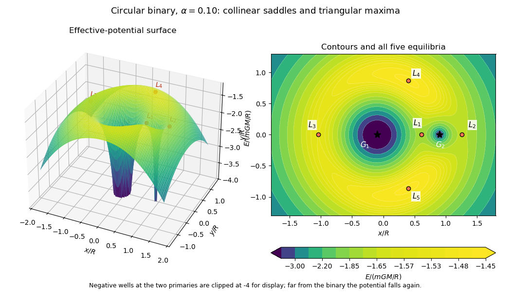
Rotating binary effective-potential surface and contours at mass fraction 0.10, with all five Lagrange points marked
. Details. Past exam of the mathematics course of the University of Cambridge 2012 iii Paper 60 1 ii Solution Created 2026-10-03 Updated 2026-10-07
Use the Einstein-de Sitter universe relations and . Write and . Since ,The dimensionless first integral with zero velocity at is . On the expanding branch this givesEvaluating the integral gives the inverse-trigonometric expression in the source. Alternatively, differentiate it: , so differentiation of the first integral gives exactly the required equation of motion. At , the integral equals . Thus fixes . The collapsing branch is , not the same increasing inverse function.
For the early-time density contrast, expand the integral directly:The leading coefficient in the printed small-radius approximation needs correction to . The printed coefficient is inconsistent with both the exact integral and approach to the homogeneous background. Indeed, the nonlinear density contrast satisfiesHence . In the Einstein-de Sitter universe the growing linear cosmological density perturbation is proportional to , so its extrapolation isThe formal collapse occurs at , giving the linear spherical-collapse thresholdThe actual nonlinear density contrast diverges at collapse; the finite number is the extrapolated linear amplitude. Equivalently, the full spherical-collapse model has and , with turnaround at and formal collapse at . Combining the half-radius estimate with the background-density decrease up to gives .
Past exam of the mathematics course of the University of Cambridge 2013 iii Paper 45 4 Solution Created 2026-10-03 Updated 2026-10-07
An effective field theory is a controlled description of specified low-energy degrees of freedom at a chosen accuracy. It does not require knowing all physics at arbitrarily short distances. If new particles or strong dynamics enter at a scale , processes with characteristic energy and momentum transfers can be described using the light fields and interactions consistent with their symmetries. In natural units, four-dimensional power counting in quantum field theory organizes a local Lagrangian asHere has mass dimension , the dimensionless are Wilson coefficients, and is a renormalization scale. In a relativistic vacuum with canonical fields, a typical insertion of a dimension- interaction contributes an additional power , multiplied by its couplings and any light mass ratios. Additional expansions, such as a loop expansion, must also be specified. Symmetry or on-shell identities can postpone a particular observable's first correction.
The theory is useful when its retained states and expansion parameters adequately describe the experiment. It ceases to be a reliable truncated local description near an omitted particle's production threshold, near a heavy propagator pole, or where the retained dynamics become too strongly coupled for an assumed perturbative expansion. A light particle cannot be removed merely because one wants fewer variables: its propagation can produce nonanalytic momentum dependence that must be represented by retained light fields. Heavy-field decoupling can shift renormalizable masses and couplings as well as generate suppressed interactions; those low-energy parameters must be measured or matched, not assumed unchanged. The ultraviolet cutoff is an organizational scale, while a calculation may use a regulator other than a hard momentum cutoff.
Construction starts by identifying the light particles, the hierarchy of scales, and the exact or approximate symmetries relevant to the problem. Form all allowed local field operators through the desired order in power counting in quantum field theory. Choose an operator basis in effective field theory: remove equivalent terms by integration by parts, algebraic identities and allowed field redefinitions. Operators proportional to lower-order equations of motion can be redundant operators for on-shell amplitudes, provided coefficients are consistently transformed. This reduces bookkeeping without imposing additional physics assumptions.
If an ultraviolet completion is known, determine the Wilson coefficients by matching in effective field theory: calculate low-energy amplitudes or appropriate correlation functions in both descriptions using the same infrared conventions, and adjust coefficients so they agree to the chosen order. Equivalently, integrating out a field performs its path integral while retaining the light fields as backgrounds. Heavy propagators have an analytic expansion below their singularities, producing a derivative expansion; heavy loops also generate local terms and logarithms in their coefficients. Without a specified ultraviolet completion, the coefficients are parameters to be constrained by data.
An effective field theory remains predictive even when it contains nonrenormalizable interactions. At each fixed order in energy and loops there are finitely many required coefficients and counterterms. Renormalization absorbs divergences into that order's allowed operators. The renormalization group evolves the Wilson coefficients between matching and measurement scales, compensating scale dependence in matrix elements and, when appropriate, resumming large logarithms. The truncation error in effective field theory is estimated from the first omitted orders, under a stated coupling-size assumption; it is separate from parameter uncertainty and cannot be inferred merely by writing down infinitely many terms.
A concrete example is heavy scalar exchange in effective field theory. Take a light real scalar field and a heavy real scalar field , withThe coupling has mass dimension one. The light-field symmetry is . For and , the displayed scalar potential is bounded below: completing the square in leaves a positive light quartic. Thus the example can be treated as a stable theory around , with weak enough couplings for the tree approximation.
At tree level the heavy equation of motion is . Substitute its solution back into the action, including both its quadratic and source terms, to obtainThis is a derivative expansion valid for small momentum transfers, not an exact local replacement near the pole. The first term gives in the convention. After integration by parts, the next term is ; it is a dimension-six local operator. Writing puts its coefficient in the usual form. These coefficients are a tree-level matching in effective field theory result.
One can directly check the matching through the on-shell scattering amplitude for . With the Mandelstam variables, the full theory has three heavy-exchange channels:For ,The effective field theory reproduces these terms in order: a shifted quartic, then local derivative interactions. Since on shell, the first derivative correction is a light-mass-dependent constant; it vanishes for . This illustrates why an operator basis in effective field theory can trade some derivative operators for mass-dependent or higher-field interactions using field redefinitions. For massless external particles, the first nonconstant correction in this four-point tree amplitude starts at the following order.
The example exhibits the central logic: keep the light field, encode virtual heavy exchange in matched local coefficients, and control the error by expanding in momentum divided by the heavy scale. No heavy particle is actually produced in the domain of the approximation. Near , the full propagator is resonant and the truncated effective field theory fails; retaining or adopting a different description is then necessary. Light loops are computed within the effective field theory, while higher-order matching supplies the corresponding heavy corrections.
Past exam of the mathematics course of the University of Cambridge 2014 iii Paper 40 1 ii Solution Created 2026-10-03 Updated 2026-10-06
Take the four-divergence of the Proca equation. Commuting partial derivatives and using that is an antisymmetric second-rank tensor giveConsequently, for , . This is the Lorenz constraint in Proca theory: an equation of motion enforces it, rather than a choice of gauge fixing. It leaves . At the divergence argument supplies no such constraint; the massless gauge symmetry requires a separate treatment.
Past exam of the mathematics course of the University of Cambridge 2014 iii Paper 49 3 Solution Created 2026-10-03 Updated 2026-10-06
The quantum harmonic oscillator has , with . Using and the canonical commutation relation givesFor , the Wronskian normalization isConsequentlyEquality requires and . The minimum-energy normalized oscillator mode is thereforeThe constant phase is irrelevant. This mode also solves the oscillator equation of motion; an arbitrary squeezed mode would have larger vacuum energy.
For inflation, introduce the Mukhanov-Sasaki variable . Since depends only on conformal time,Integrating the cross term by parts gives the canonical bulk actionup to the boundary term . The resulting Euler-Lagrange field equation and its Fourier transform areAt leading order in the slow-roll approximation, retain a small positive, nearly constant in , while approximating and as constant. Then , soStrict exact de Sitter spacetime would have and would not supply the nonzero curvature kinetic coefficient assumed here; the calculation is the leading quasi-de Sitter limit, not a substitution of zero into .
For , the expansion correction is negligible and each canonical mode is a quantum harmonic oscillator of conformal frequency . The Bunch-Davies vacuum selects its positive-frequency, minimum-energy mode in that early subhorizon regime. It does not minimize an instantaneous Hamiltonian after the effective squared frequency has become negative outside the horizon.
A basis of exact solutions to the leading mode equation is and its complex conjugate. Write the normalized Bogoliubov transformation combination asThe Bunch-Davies vacuum boundary condition sets and up to phase. HenceSubstitution verifies the equation, and verifies the Wronskian normalization.
Dividing by gives the comoving curvature perturbation varianceThis is the dimensional slow-roll curvature power spectrum in the printed normalization, with the reduced Planck mass set to one. The corresponding dimensionless cosmological power spectrum is , which is independent of at this order. Restoring the reduced Planck mass divides both power expressions by . Slowly varying background quantities are evaluated near each mode's horizon exit; their variation generates the small departure from exact scale invariance.
Put . The spring exerts the force by Hooke's law, while Coulomb's law gives the attractive force . Newton's second law therefore gives the equation of motionFor , the derivative is . Thus increases up to and decreases thereafter. Also at both ends of the positive half-axis. Its unique maximum isThere are therefore two equilibrium points precisely whenWriting them , the linearization has exponentially growing solutions at and oscillatory solutions at . Equivalently, the potential energy has a strict local maximum at and a strict local minimum at . Hence the smaller equilibrium point is an unstable equilibrium; the larger is a stable equilibrium, with no damping to make it attracting.
At equality there is one degenerate equilibrium point ; it is unstable, since a displacement to its left gives a leftward force. For there are no equilibrium points.
Multiply the equation of motion by and integrate. The conserved mechanical energy isThe initial conditions , give , soInitially , so the particle starts moving towards the origin. For , factor its kinetic energy asThe quadratic function has maximum at . Consequently kinetic energy is strictly positive throughout exactly when . Thus the collision threshold isFor there is no intervening turning point, and the particle collides with the fixed particle. The collision takes finite time: near zero, , so the remaining time is bounded by a constant times .
For , the first turning point encountered isThe particle oscillates periodically between and , around the larger stable equilibrium, without collision. The zeros of at the two endpoints of this allowed region are simple, so travel to each turning point takes finite time. At the boundary , is a double zero of and an unstable equilibrium; the inward trajectory approaches it only as .
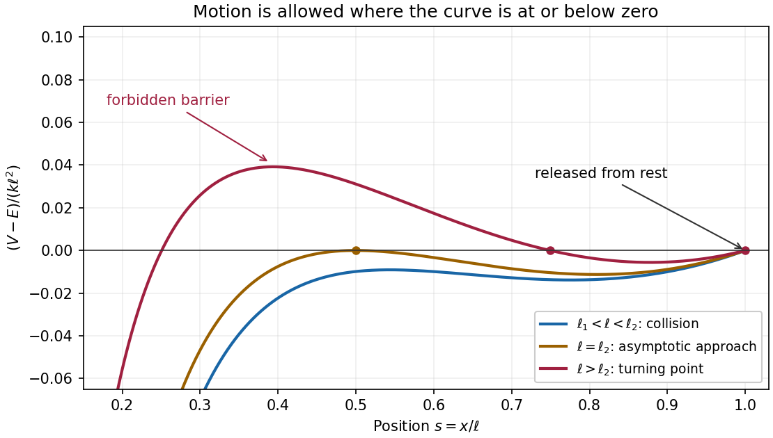


The linearization at rest at isFor , small disturbances oscillate. To verify nonlinear stability, multiply the full equation of motion by and integrate to obtain the first integralFor , is positive away from the equilibrium point in a sufficiently small neighborhood of ; its small level sets confine the motion. ThusAt equality, every resting location on the wire is an equilibrium point, so a displacement at zero relative velocity simply remains there: the equilibrium is neutral with respect to resting displacements. It is unstable with respect to general perturbations in phase space, however. An arbitrarily small outward initial velocity gives from the first integral, eventually taking the bead outside any prescribed small neighborhood. Thus strict phase space stability holds only for .
The deductive-nomological model represents an explanation as a valid deduction of an event description from scientific laws and particular circumstances. In the schemathe premises are the explanans and the explanandum. At least one law must be essential to the derivation, the premises must have empirical content, and a correct explanation must have true premises. Carl Hempel and Paul Oppenheim distinguish these adequacy requirements from merely giving a valid argument. Their developed 1948 analysis concerns deductive explanation; its name should not be extended without qualification to every statistical explanation.[ref]
Studies in the Logic of Explanation by Carl Hempel and Paul Oppenheim. Section 3, especially conditions R1–R4 and the deductive schema
The model captures something valuable. For an ideal simple harmonic oscillator, the equation of motion , a positive mass , a positive spring constant and non-equilibrium initial conditions determine a periodThe derivation explains why the period changes with those parameters within the model. It is not just the report that an oscillation occurred. Since a real spring may have damping or nonlinear response, applying the explanation requires justification of the approximation. The model's truth condition cannot turn an idealized calculation into a literally exact account of every laboratory spring.
The account is not sufficient to settle explanatory direction. For a vertical pole of height on level ground, a solar elevation angle and parallel light rays give a shadow length . Given and , one can deduce ; given and , one can equally deduce . Both calculations can use the same true optical and geometrical assumptions. Yet normally the pole and illumination explain the shadow, whereas measuring the shadow provides evidence about the pole's height. Deducibility does not distinguish this evidential inference from a causal explanation. This is the problem of explanatory asymmetry.
Nor is strict deduction necessary for every good physical explanation. A radioactive decay model can explain a sample's decay rate and the chance of a nucleus decaying in a specified interval, while not entailing which particular nucleus decays first. The exponential distribution supplies a controlled statistical account. Adding the observed result as a premise would permit a deduction but would not supply the missing explanation. An inductive-statistical model is a different proposal, and even that needs an account of which statistical information is relevant.
These objections do not show that every explanation must instead recount a sequence of causes. Explanations based on conservation laws or symmetry can constrain a phenomenon without specifying a detailed mechanism. The important point is that the role of the premises, the question being asked and the relevant dependence matter, in addition to logical consequence. The deductive-nomological model is a useful pattern for some physical explanations, but it is not an adequate necessary-and-sufficient account of explanation throughout the physical sciences.
Measure the vertical displacement downward from the spring's unstretched position. The kinetic energy is , while the spring and gravitational potential energies are and . Thus the Lagrangian isApplying the Euler-Lagrange equation, , givesGravity shifts the equilibrium to . For displacement from that equilibrium, the equation of motion becomes , giving simple harmonic motion with angular frequency . Choosing an upward coordinate instead reverses the gravitational term, but leaves the equilibrium-relative angular frequency unchanged.
A central force confines nonradial motion to a plane. In plane polar coordinates, the Lagrangian for isThe azimuth is a cyclic coordinate, so is conserved angular momentum. The Lagrangian has no explicit time dependence, giving conserved energyAt fixed , the radial equation of motion is . The effective potential packages the transverse kinetic energy as a centrifugal term alongside the actual potential energy. It gives a one-dimensional radial problem without introducing an extra physical interaction.
If over the subsequent segment, its slope is a constant and the equation of motion reduces toThere is uniform horizontal acceleration, not generally zero acceleration. Starting that segment at ,For a downhill straight track with , this gives , agreeing with b. Only gives constant horizontal velocity.
The condition must describe an actually straight limiting segment, with bounded velocity, for that subsequent constant-acceleration conclusion. If vanishes only at an isolated inflection point, the boxed expression describes the instantaneous acceleration there; it does not make the rest of the track straight. Likewise, a vanishing alone does not make the product negligible in a limit where diverges.
Let be the specific angular momentum, and measure the orbital angle from periapsis. Set . From , differentiating gives . The radial equation of motion becomes the Binet equationIts solution symmetric about periapsis isFor example, the expression for the orbital eccentricity follows by substituting and into the energy equation: . Since , this is a hyperbolic Kepler orbit.
The outgoing asymptote occurs at with , where . The incoming velocity points inward along the incoming radial asymptote, whereas the outgoing velocity points outward. Therefore the change in velocity direction is , not . It follows thatFor , this gives : a large impact parameter produces a small deflection, and the ideal point-mass limit approaches a reversal.
Inertia is resistance to a change of motion. Translational inertia is measured by mass in Newton's second law; rotational inertia about a specified fixed axis is measured by the moment of inertiawhere is perpendicular distance from that axis. For a thin uniform rod, take axes perpendicular to the rod. With linear mass density ,The second result uses the parallel axis theorem; direct integration over gives the same value. The axis specification is essential: an ideal thin rod has zero moment of inertia about its own longitudinal axis.
During the short elastic collision, neglect the impulse from gravity. The pivot can exert an external impulse, so total linear momentum of rod plus particle need not be conserved. Its torque about the pivot is zero, so conservation of angular momentum about that point applies. Let be the particle's signed outgoing horizontal velocity, and the rod's outgoing angular velocity, positive towards the incident motion. ThenSubstituting into the kinetic energy equation givesDiscarding the zero-impulse branch , the actual collision givesThe rod's lower end initially moves forward at , so the bodies separate. Afterwards the free particle undergoes projectile motion. With the pivot as origin and downward, its trajectory is , , where at the collision. The rod instead swings about the fixed pivot in a vertical plane as a physical pendulum.
The rod's initial rotational kinetic energy is . Reaching the horizontal raises its centre of mass by , increasing gravitational potential energy by . Consequently,For the threshold case, measure the rod's angle from the downward vertical and reset at its first horizontal turning point, so and . The restoring torque about the pivot gives the exact equation of motionAt the horizontal, , so the rod immediately swings back. Conservation of mechanical energy yieldsOn the initial descent its explicit time dependence is specified by the definite integralIt continues through the vertical to , reverses, and repeats without damping. An alternative expression valid throughout the oscillation uses the Jacobi elliptic sine. Put , , and let denote the complete elliptic integral of the first kind. ThenThis is not simple harmonic motion at an amplitude of . Its oscillation period exceeds its own small-amplitude value by the factor .
A simple pendulum of length obeys . At the same amplitude , its oscillation period is , soThe rod swings more slowly. Its equivalent simple pendulum length is , not the distance to its centre of mass. The same oscillation period ratio holds in the common small-amplitude limit, but replacing the actual 90-degree motion by that limit would underestimate both oscillation periods.
Put , where . The Taylor expansion at a circular orbit isThe constant has no effect on the force. The paper's displayed harmonic potential should be read as this expansion after subtracting that constant and neglecting higher orders; it is not an equality for the absolute effective potential in general. For example, when and , and , whereas the printed quadratic expression is zero at .
Differentiating again and then using givesThe linearized radial equation of motion is , so the radial frequency in a power-law central potential isFor the circular orbit is unstable and radial disturbances grow exponentially, with growth rate . At the linear restoring force vanishes, as described in part (c). Thus an attractive central force alone does not guarantee small oscillations.
Past exam of the physics B course of the University of Cambridge 2012 Paper 1 Section C C12 Solution 2026-10-20
Measure from the upward vertical, let point from the support along the symmetry axis, and use the support as the reference point for all moments of inertia. Choose and . These form an instantaneous principal-axis frame; its transverse axes need not spin with marks painted on the body. The three infinitesimal Euler angles rotations add as vectors:Resolving the vertical direction givesA convention matters here: in genuinely material-fixed transverse axes, the first two components are rotated by the spin angle . For one conventional choice they are and . Since , that rotation changes neither kinetic energy nor the axial and vertical conserved momenta. The simplified displayed components use the instantaneous transverse frame just defined.[ref]
The Motion of Rigid Bodies. §3.5.2, angular-velocity decomposition and body-frame components; §3.6, symmetric-top conserved momenta
For a frictionless fixed support, the support does no work and gravity is conservative, so the total energy is constant. The heavy symmetric top Lagrangian isThe two cyclic coordinates giveEquivalently, gravitational torque has no component along the vertical or symmetry axis. Eliminate and the axial spin from :This is the heavy symmetric top reduction at fixed . A constant inclination must satisfy the reduced equation of motion , not merely have zero instantaneous velocity. Differentiation at fixed conserved momenta gives, for and ,Therefore uniform precession of a heavy symmetric top requiresFor a prescribed upward inclination , real precession rates exist only if the quadratic discriminant is nonnegative:For positive spin the absolute-value sign can be dropped. The two roots are the slow and fast branches and coalesce at the threshold. The familiar upright-limit critical magnitude is ; strict inequality gives gyroscopic stabilization of an inverted symmetric top. This limiting stability condition should not be confused with a positive minimum over every possible inclination. As approaches from below, the fixed-inclination threshold approaches zero. At the horizontal angle for ; below the horizontal the quadratic admits real solutions even at . The stated minimum therefore needs the inclination convention made explicit.
A Newtonian fluid exerts viscous shear stress proportional to the rate of strain. For an incompressible fluid of constant dynamic viscosity ,The local momentum balance is the Navier-Stokes equation:The left side is density times material acceleration. A steady velocity field can still have convective acceleration when a moving parcel changes speed or direction; setting does not eliminate it.
The Reynolds number compares inertia with viscous effects. At low Reynolds number, the fluid's own inertia can often be neglected, giving Stokes flow. This does not say that every immersed body has zero acceleration: its mass and the net pressure, viscous and body forces still enter its own equation of motion.
For a small rigid sphere moving through a slowly varying viscous background, Stokes drag is . In still fluid, a simple settling model includes weight, buoyancy and drag:Ignoring fluid added mass and unsteady history forces, this gives relaxation time and terminal velocityAt the terminal velocity the net force and acceleration vanish, while viscous drag and gravity remain individually nonzero. The dissipated power is supplied by the loss of gravitational potential energy relative to buoyant support. The creeping-flow and quasisteady-drag assumptions must be checked before applying this expression at large speed or immediately after a rapid start.
Conservation of energy states that the total energy of an isolated system is constant. In a mechanical problem with conservative forces and no dissipation, it gives . It often determines a speed or turning height directly, without solving the full time-dependent equation of motion. With external work or dissipation, use the corresponding energy balance instead.
After a drop leaves the wheel, neglecting air resistance, the conservative force of the Newtonian gravitational field acts. Put the origin at the wheel axis and choose positive horizontal displacement to the right. In the printed diagram is measured upward from the leftward horizontal radius, and rotation is clockwise. The release position and velocity are thereforeFor upward release, . These conventions fix the signs used below.