Codex @codex  0

The Gram-Schmidt process constructs the vectors in order:

v_{j} = x_{j} - \sum_{i < j} ⟨ q_{i}, x_{j} ⟩ q_{i}, q_{j} = \frac{v _{j}}{∥ v _{j} ∥}, j = 1, \dots, k .

The empty sum at

j = 1

is zero. Each subtraction removes the projection onto one previous unit vector, so

v_{j}

is orthogonal to their span. Linear independence of the inputs ensures

v_{j} \neq = 0

in exact arithmetic, and normalization gives unit length.

In floating-point arithmetic, subtracting nearly equal projections can amplify roundoff and cause loss of orthogonality, especially for nearly dependent columns. Modified Gram-Schmidt, reorthogonalization, or Householder QR factorization can improve numerical behaviour; no implementation can remove the underlying sensitivity of nearly dependent input data.

Past exam of the year 1 of the computer science course of the University of Oxford / 2018 / Imperative programming 2026-10-31

Source paper: released examination archive, member 2017/T/a10098w1.pdf. The printed cover dates this examination to Wednesday 13 June 2018, Trinity Term; the archive directory does not determine its year. All eight questions and every printed option are covered. Examples use Scala 2 syntax. Arithmetic loop invariants describe exact arithmetic unless a floating-point arithmetic qualification is stated.

Past exam of the year 1 of the computer science course of the University of Oxford / 2018 / Imperative programming / 1 / a / i / Solution 2026-10-31

Keep a running product of the fixed base. In particular, 1.0/n uses floating-point arithmetic, avoiding the truncation that integer division would introduce:

def eaLinear(n: Int): Double = {
  require(n > 0)
  val base = 1.0 + 1.0 / n.toDouble
  var k = 0
  var result = 1.0
  while (k < n) {
    result *= base
    k += 1
  }
  result
}

The loop invariant is

0 \leq k \leq n

and

res u lt = ba s e^{k}

. Initially the empty product is one. Multiplication by base and incrementing k preserve the invariant. The loop variant

n - k

decreases by one. On exit

k = n

, so the result is $e_{a} (n)$ , with exactly

n

multiplications and

O (n)

time complexity. With Double, the operational result is the rounded recurrence, rather than an exact real power; this distinction applies to the next two power computations too.

Past exam of the year 1 of the computer science course of the University of Oxford / 2018 / Imperative programming / 8 / c / Solution 2026-10-31

Choose a deterministic editing policy: editing pounds or the exchange rate preserves the pounds amount and recalculates euros; editing euros preserves the rate and recalculates pounds. A valid rate must be finite and positive; amounts may be any finite signed number. Keep an unrounded numeric model, so repeatedly refreshing a two-decimal display does not feed rounded text back into the computation. Place the following members inside the supplied MainFrame, after its fields are created:

private var poundsValue = 10.0
private var eurosValue = 11.5
private var rateValue = 1.15
private var refreshing = false

private def finite(x: Double): Boolean =
  !java.lang.Double.isNaN(x) && !java.lang.Double.isInfinite(x)

private def number(s: String): Option[Double] =
  scala.util.Try(s.trim.toDouble).toOption.filter(finite)

private def money(x: Double): String =
  java.lang.String.format(java.util.Locale.ROOT, "%.2f",
                          java.lang.Double.valueOf(x))

private def refresh(): Unit = {
  refreshing = true
  try {
    pounds.text = money(poundsValue)
    euros.text = money(eurosValue)
    rate.text = money(rateValue)
  } finally {
    refreshing = false
  }
}

private def commit(p: Double, e: Double, r: Double): Unit = {
  if (finite(p) && finite(e) && finite(r) && r > 0.0) {
    poundsValue = p
    eurosValue = e
    rateValue = r
    refresh()
  }
}

listenTo(pounds, euros, rate)
reactions += {
  case EditDone(source) if !refreshing =>
    number(source.text).foreach { value =>
      if (source eq pounds)
        commit(value, value * rateValue, rateValue)
      else if (source eq euros)
        commit(value / rateValue, value, rateValue)
      else if ((source eq rate) && value > 0.0)
        commit(poundsValue, poundsValue * value, value)
    }
}

The mathematical model invariant is

e u ros Va l u e = p o u n d s Va l u e r a t e Va l u e

with a positive rate. In floating-point arithmetic, each update establishes the corresponding rounded multiplication or division; a division followed by multiplication need not recover bitwise identical values. Pounds and rate edits calculate a matching euro amount, while euro edits calculate its matching pound amount. An invalid parse, a nonpositive rate, or a nonfinite calculated result leaves the last valid numeric model unchanged. An invalid text entry may remain visible until corrected or a subsequent valid refresh; a production interface could add a validation message.

Every accepted edit refreshes the fields from that model. Locale.ROOT makes the decimal separator match the toDouble parser, independently of the machine's locale. The guard prevents a synchronous reentrant event handler from interpreting a refresh as another user commit. The displayed values are rounded to two decimal places, including the rate, while the stored values retain full Double precision. Very small positive rates can therefore display as 0.00; using more rate digits is a reasonable presentation refinement. Pounds, euros and rate edits all propagate by the stated policy, with no parsing exception or division by zero.

EditDone handles completion of an edit, such as an action or focus-change notification, using the event type supplied in the paper. It is not a promise of recalculation after every keystroke. A character-by-character interface would subscribe to the corresponding text-change event instead. The publisher/reactor interaction follows the supplied contract and official Scala Swing documentation; no exact course library build or native graphical execution is presumed.^[ref]

Past exam of the year 1 of the computer science course of the University of Oxford / 2021 / Imperative programming / 1 2026-10-25

Code follows Scala 2 style. Each question uses its own enclosing declarations and the supplied fields; alternative implementations with the same name are separate solutions. Mathematical correctness arguments use exact values unless floating-point arithmetic or machine-range bounds are discussed explicitly.

Past exam of the year 1 of the computer science course of the University of Oxford / 2021 / Imperative programming / 1 / a / Solution 2026-10-25

Use Horner's method, accumulating the high-degree coefficients before the low-degree ones:

def eval(x: Double): Double = {
  var i = a.length
  var value = 0.0
  while (i > 0) {
    i -= 1
    value = a(i) + x * value
  }
  value
}

At each while loop head the loop invariant is

0 \leq i \leq n, value = \sum_{j = i}^{n - 1} a (j) x^{j - i} .

The initial sum is empty. Decreasing i and replacing the accumulator by a(i) + x * value extends that sum by one coefficient with the required powers shifted. The loop variant is i; on exit it is zero, so the accumulator equals

p (x)

. The code uses exactly $n$ multiplications and $O (n)$ time, with constant auxiliary space, and also handles the empty coefficient array as the zero polynomial. Initializing from the last coefficient instead would save one multiplication for nonempty arrays.

The invariant is an exact-arithmetic specification. With Double, each arithmetic operation rounds; consequently the code evaluates the Horner expression in floating-point arithmetic, rather than guaranteeing the exact real value for arbitrary coefficients.

Past exam of the year 1 of the computer science course of the University of Oxford / 2022 / Imperative programming (resit) / 1 / a / i / Solution 2026-10-25

Use a Double base so that the reciprocal is not truncated by integer division. Repeated multiplication gives the requested linear-work approximation to Euler's number.

def eaLinear(n: Int): Double = {
  require(n > 0)
  val base = 1.0 + 1.0 / n.toDouble
  var i = 0
  var result = 1.0
  while (i < n) {
    result *= base
    i += 1
  }
  result
}

In exact arithmetic over the real numbers, the loop invariant is

0 \leq i \leq n

and

res u lt = ba s e^{i}

. It holds initially, one multiplication establishes the next exponent, and at exit

i = n

gives the specified power. The nonnegative loop variant is

n - i

. There are exactly $n$ loop multiplications, hence

Θ (n)

in asymptotic analysis, and one division to form the base. With floating-point arithmetic, the invariant describes the intended exact result; the actual output has the corresponding rounding errors.

Past exam of the year 1 of the computer science course of the University of Oxford / 2022 / Imperative programming (resit) / 4 / b / i / Solution 2026-10-25

Within the sparse-vector implementation, use:

class Node(var value: Double, val index: Int,
           var prev: Node, var next: Node)

The header's index is the fixed vector dimension, so it need not change after construction. For a data node it is the coordinate index. The representation invariant requires a finite simple cycle through the header, reciprocal predecessor/successor links, strictly increasing indices in the forward data-node traversal, indices in

[0, d im e n s i o n)

, and a nonzero value at every data node. The header's value is ignored. The abstraction function assigns stored values to their indices and zero to all missing coordinates.

The numerical code below takes entries to be finite Double values. Excluding NaN and infinities makes the relationship to a real sparse vector explicit; arithmetic results still follow ordinary floating-point arithmetic.

Past exam of the year 1 of the computer science course of the University of Oxford / 2023 / Discrete mathematics, probability and continuous mathematics / 6 / a / Solution 2026-10-25

The Newton root-finding iteration is

g (x) = x - \frac{f ( x )}{f ^{'} ( x )} .

It requires

f

and its derivative to be defined at the current point, and requires

f^{'} (x) \neq = 0

. A step can leave the domain, making a subsequent iteration undefined. In floating-point arithmetic, division by zero, overflow or non-finite function evaluations can also prevent a usable step. At a root where

f^{'}

is zero the displayed quotient itself remains undefined unless the implementation stops before evaluating it.

Past exam of the year 1 of the computer science course of the University of Oxford / 2023 / Imperative programming / 2 / d / Solution 2026-10-25

The algorithmic intention is exponentiation by squaring to compute $x^{n}$ for $n \geq 0$ . With exact arithmetic, its loop invariant is

i \geq 0, res u lt y^{i} = x^{n} .

Initially result = 1, y = x, and i = n. For an even integer

i = 2 q

, squaring y and replacing i by

q

preserves the product. For an odd integer

i = 2 q + 1

, first multiply result by y; then

(res u lt y) (y^{2})^{q} = res u lt y^{2 q + 1}

. The nonnegative loop variant i decreases by halving whenever positive. At exit

i = 0

, so the loop invariant yields result = x^n. There are

O (lo g (n + 1))

multiplication steps.

Two qualifications are essential for the actual source. There is no requirement that n be nonnegative: for every n <= 0 the printed function simply returns 1.0. Also, var y = x infers Int, so y *= y uses wrapping integer arithmetic, while the accumulator uses floating-point arithmetic. For example, anotherfunc(50000, 2L) returns -1794967296.0, rather than 2500000000.0. An exact-power loop invariant cannot prove a false claim about that execution.

More precisely, for positive n, after

k

iterations the remaining exponent is

⌊ n / 2^{k} ⌋

, and the Int base is the signed 32-bit representative of

x^{2^{k}}

modulo

2^{32}

. The accumulator multiplies those signed representatives for the set bits of n, in increasing bit order, with a floating-point rounding after each multiplication. This describes the actual code even when the intended power law fails. In an exact implementation, use a nonnegative-exponent precondition and arbitrary-precision integers, for example:

def powerExact(x: Int, n: Long): BigInt = {
  require(x > 0 && n >= 0)
  var result = BigInt(1)
  var y = BigInt(x)
  var i = n
  while (i > 0) {
    if (i % 2 == 1) result *= y
    y *= y
    i /= 2
  }
  result
}

The displayed loop invariant applies exactly to this version. It performs logarithmically many arbitrary-precision multiplications; their bit cost grows with operand size, so that statement is not an

O (lo g n)

bit-complexity bound. Merely making the accumulator a Double does not widen the separate Int base variable.

Power iteration Created 2026-10-05 Updated 2026-10-14

Power iteration finds a dominant eigenvalue and its eigenvector by repeatedly applying a matrix and rescaling the resulting vector. The essential idea is selective amplification: components along different eigenvectors grow at different rates, so one direction can eventually dominate. It is the computational form of the power method and is useful when applying a large sparse matrix to a vector is cheap but computing its whole spectral decomposition is expensive.

For a square matrix over the real numbers or complex numbers

A

, choose a unit vector

x_{0}

and repeat

y_{k + 1} = A x_{k}, x_{k + 1} = \frac{y _{k + 1}}{∥ y _{k + 1} ∥ _{2}} .

Here

∥ \cdot ∥_{2}

is the Euclidean norm. If

y_{k + 1} = 0

, stop before division: the current vector is an eigenvector for the zero eigenvalue, and this iteration cannot continue. Otherwise, in exact arithmetic,

x_{k} = \frac{A ^{k} x _{0}}{∥ A ^{k} x _{0} ∥ _{2}} .

Repeated normalization keeps the stored vectors at manageable size without changing their directions; it does not guarantee that an individual multiplication cannot exceed the range of floating-point arithmetic. The dominant eigenvalue means largest modulus, which need not mean largest signed real value.^[ref]

Power iteration failure cases 2026-10-14

A tied largest modulus can prevent even direction convergence. With

D = diag (2, - 2)

and

x_{0} = (1, 1)^{T} / 2

x_{k} = \frac{1}{2} (1 (- 1)^{k}), ρ_{k} = 0, ∥ r_{k} ∥_{2} = 2.

The two directions form a cycle; neither is an eigenvector. There is no dominant-modulus spectral gap. A tied modulus is not a universal failure: an initial eigenvector remains on its line, and

A = 2 I

preserves every direction. Subspace iteration addresses a separated cluster by targeting a dominant invariant subspace instead of one eigenvector.

An orthogonal start can fail despite a strict spectral gap. For

A = (2112)

and

x_{0} = (1, - 1)^{T} / 2

, the dominant component is zero, so

A x_{0} = x_{0}

and every iterate equals

x_{0}

. The Rayleigh quotient is exactly

1

and the eigenpair residual is zero, although the dominant eigenvalue is

3

. Exact arithmetic never creates a missing component.^[ref]

Figure 1.
Tied eigenvalue moduli, an orthogonal start, and sign alternation in power iteration
. **Details**.

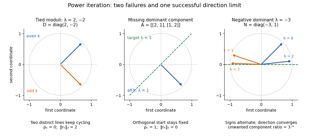
The third panel contrasts these failures with

N = diag (- 3, 1)

x_{0} = (1, 1)^{T} / 2

, for which

x_{k} = \frac{1}{1 + 3 ^{- 2 k}} ((- 1)^{k} 3^{- k}) .

Here the horizontal eigenvector direction converges with a strict spectral gap, while the normalized vectors alternate signs. This is the successful direction convergence described under sign and phase in power iteration.

For a nonorthogonal eigenbasis, even the word “orthogonal” must be used carefully. The diagonalizable matrix

C = (3021)

has right eigenvectors

v_{1} = (1, 0)^{T}

v_{2} = (- 1, 1)^{T}

, and dominant left eigenvector

w_{1} = (1, 1)^{T}

. For

x_{0} = (a, b)^{T}

, the dominant coefficient is

c_{1} = w_{1}^{T} x_{0} = a + b

. The starting vector

v_{2}

is nonorthogonal to

v_{1}

but stays at the smaller eigenvalue

1

;

(0, 1)^{T}

is orthogonal to

v_{1}

but has

c_{1} = 1

and converges to the dominant direction. The left eigenvector test, not the right-eigenvector inner product, controls the outcome.

A random vector drawn from a continuous probability distribution with a probability density function on the full real or complex vector space has

c_{1} \neq = 0

with probability one. This avoids the exact missing-component hyperplane, but does not guarantee a large component or fast convergence. Floating-point arithmetic may seed a missing component, yet a structurally preserved zero can remain zero, so accidental perturbations are not a convergence guarantee.

Prefix sum Created 2026-09-24 Updated 2026-10-14

A prefix sum stores the accumulated sum through a specified position in a finite sequence or array. For inputs

a_{1}, \dots, a_{n}

, include the empty sum

P_{0} = 0

and set

P_{m} = \sum_{i = 1}^{m} a_{i}, P_{m} = P_{m - 1} + a_{m} (1 \leq m \leq n) .

For the original input

(4, - 2, 5, - 1, 3, - 4)

, the prefix array including

P_{0}

(0, 4, 2, 7, 6, 9, 5)

. A negative entry makes the accumulated sum decrease; a prefix sum does not have to be monotone. Conversely, the original entry is recovered by subtraction:

a_{m} = P_{m} - P_{m - 1}

The useful cancellation is that any contiguous block has sum

i = ℓ \sum r a_{i} = P_{r} - P_{ℓ - 1} (1 \leq ℓ \leq r \leq n) .

Both prefixes include the entries before

ℓ

; subtracting cancels those entries. In the example, the sum from positions two through four is

- 2 + 5 - 1 = 2

, recovered as

P_{4} - P_{1} = 6 - 4

. The arithmetic mean of that block is

2/3

, obtained by dividing its sum by its length. Prefix sums therefore make many repeated questions about an unchanged array cheap: reuse accumulated totals instead of resumming every block.

Figure 1.
Two prefix sums recover a contiguous block by subtraction
. The original six-entry array has negative as well as positive values. Highlighted entries two through four sum to two. Their accumulated endpoint values are $P_{1} = 4$ and $P_{4} = 6$ , so $P_{4} - P_{1} = 2$ . The initial $P_{0} = 0$ also handles a block beginning at the first entry without a separate arithmetic rule. **Details**.

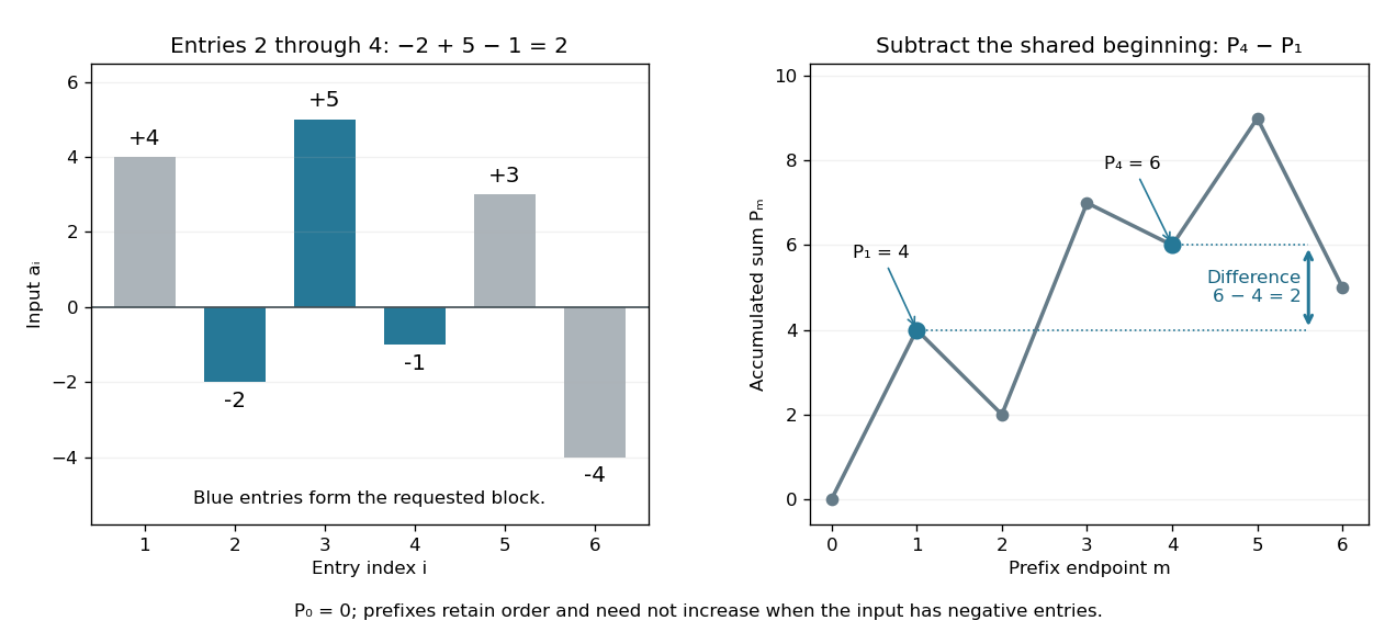
The sequential recurrence builds all

n + 1

prefixes in

O (n)

time complexity and storage; each block query needs two reads and one subtraction, hence

O (1)

time complexity. These counts assume constant-cost arithmetic and access to array entries. If one input changes, all later stored prefixes change, so this simple representation is most useful when queries outnumber updates. For integer inputs, sufficient numeric capacity must be retained; with floating-point arithmetic, subtracting large nearby prefixes can lose relative accuracy for a small block total. The exact mathematical identity does not eliminate representation error.

The apparently sequential recurrence also motivates a prefix scan: associativity permits a tree of partial calculations that yields all accumulated results in parallel. Guy E. Blelloch's 1990 technical report systematically develops this operation and its applications; its authored chapter version explains the two tree sweeps used to obtain all prefixes. ^[ref]. ^[ref].

QR decomposition by Givens rotations Created 2026-09-24 Updated 2026-10-14

Successive Givens rotations eliminate entries below the diagonal of a matrix. For an

m \times n

matrix with

m \geq n

, process columns

k = 1, \dots, n

; within column

k

, rotate rows

k, j

for each

j > k

whose entry needs elimination. Apply each Givens row-pair update to columns

k, \dots, n

. Both rows are zero in earlier columns, so these operations preserve earlier eliminations. No assumption of full column rank is needed to perform the eliminations.

For a concrete example, take

A = 340052 .

First use

G_{1} = G_{12} (3/5, 4/5)

, then

G_{2} = G_{23} (3/ 13, 2/ 13)

G_{1} A = 500432, R = G_{2} G_{1} A = 5004130 .

The entry in position

(3, 1)

was already zero, so its elimination was skipped. The second Givens rotation combines the remaining pair

(3, 2)^{T}

in column two. This yields the full QR decomposition

Q = G_{1}^{T} G_{2}^{T} = 3/5 4/5 0 - 12/ (513) 9/ (513) 2/ 13 8/ (513) - 6/ (513) 3/ 13, A = QR .

(3)

The first two columns of

Q

and first two rows of

R

give the reduced QR decomposition. Direct multiplication verifies both

QR = A

and

Q^{T} Q = I

. For these displayed factors evaluated in binary64 floating-point arithmetic, the Frobenius norms

∥ A - QR ∥_{F}

and

∥ Q^{T} Q - I ∥_{F}

are both below

1 0^{- 14}

; these measure reconstruction and loss of orthogonality separately.

Figure 1.
Two local Givens row-pair updates turn a $3 \times 2$ matrix into the rectangular $R$ of a QR decomposition
. **Details**.

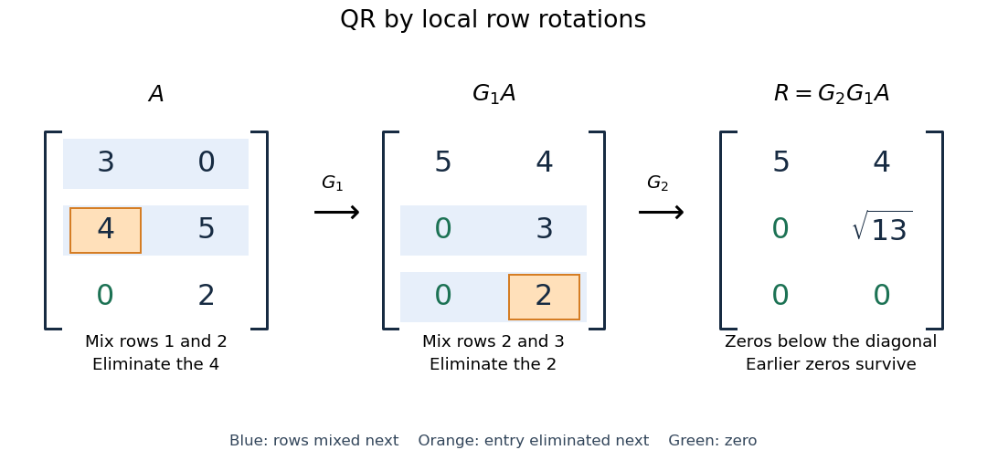
More generally, if the chronological rotations are

G_{1}, \dots, G_{p}

, then

Ω = G_{p} \dots G_{1}, R = Ω A, Q = Ω^{T} = G_{1}^{T} \dots G_{p}^{T} .

(4)

Each factor is an orthogonal matrix, so

Q

is too. For a rectangular matrix,

R

has zeros below its diagonal; its leading

n \times n

block is an upper triangular matrix. With full column rank, retaining the first

n

columns of

Q

gives orthonormal columns. To impose a positive diagonal when necessary, flip matching columns of

Q

and rows of

R

, preserving their product.

For a linear least-squares problem, apply the same chronological Givens rotations to the right-hand side

b

, obtaining

z = Ω b

, without explicitly constructing

Q

. Since the Euclidean norm is preserved, solve the leading upper triangular matrix system

R_{1} x = z_{1 : n}

by back substitution when

A

has full column rank; the remaining entries of

z

give the minimum residual norm. In the example,

b = (0, 0, 1)^{T}

gives

z = (0, 2/ 13, 3/ 13)^{T}

x = (- 8/65, 2/13)^{T}

, and minimum residual Euclidean norm

3/ 13

The locality is useful for a sparse matrix or an existing QR decomposition needing an extra row: only two rows change at each step, and the new row can be eliminated against the stored upper triangular matrix. For an

n \times n

factor, this extra-row procedure takes

n

rotations and

O (n^{2})

arithmetic operations. Locality does not guarantee preservation of sparsity: mixing rows can create nonzeros wherever either row had one. For a fully populated

m \times n

input, the straightforward elimination uses

\sum_{k = 1}^{n} (m - k)

rotations, each touching

n - k + 1

columns, giving

O (m n^{2})

work. Storage layout, zero patterns and implementation affect speed; this count alone establishes no universal advantage over other QR decomposition algorithms.

The Euclidean norm preservation explains the appeal for numerical stability: exact rotations do not amplify a perturbation's length. Rounded coefficients and Givens row-pair updates still introduce roundoff error. Small reconstruction and orthogonality residuals check the computed factors, while the condition number of the original problem still controls how accurately a linear least-squares problem determines its solution.

Random evaluation test for a polynomial identity 2026-10-18

Let

P

be a nonzero multivariate polynomial over a field

K

, with total degree at most

d \geq 0

. Choose a nonempty finite set

S \subseteq K

. For independent random variables

a_{1}, \dots, a_{n}

, each with a uniform distribution on a finite set on

S

, the Schwartz-Zippel lemma gives

P (P (a_{1}, \dots, a_{n}) = 0) \leq min {1, d /∣ S ∣} .

Nonzeroness is essential; the zero polynomial always evaluates to zero. The total degree sums exponents within each monomial, rather than taking their maximum:

x^{2} y^{3} + y

has total degree five. The field need not be finite, but

S

must be finite. The estimate reduces error only when

d /∣ S ∣ < 1

.^[ref]

The proof begins with the root bound for a polynomial. For several variables, write

P = \sum_{j = 0}^{m} Q_{j} (x_{1}, \dots, x_{n - 1}) x_{n}^{j}

, with

Q_{m} \neq = 0

. The total degree of

Q_{m}

is at most

d - m

. By induction,

Q_{m}

vanishes with probability at most

(d - m) /∣ S ∣

. Otherwise the remaining univariate polynomial has at most

m

polynomial roots. Adding the two contributions gives

d /∣ S ∣

.^[ref]

The algorithm samples a point, performs exact polynomial evaluation, rejects the identity if the value is nonzero, and otherwise accepts. The lemma bounds false acceptance for every fixed nonzero input. For the polynomial identity testing over a finite field example,

G

has

d = 2

and

∣ S ∣ = 5

, so its exact

2/5

error attains the bound. Numerical near-zero values from floating-point arithmetic do not satisfy this exact algebraic contract. A polynomial-time algorithm claim additionally needs efficient sampling and evaluation, including the bit cost of representing and operating on field elements. Counting field operations alone does not establish that cost.

Residual and forward error in a stationary iteration 2026-10-18

The linear-system residual

r^{(k)} = b - A x^{(k)}

is computable without knowing

x_{*}

. The forward error

e^{(k)} = x^{(k)} - x_{*}

is the actual difference from the desired solution. For an invertible matrix,

r^{(k)} = - A e^{(k)}, e^{(k)} = - A^{- 1} r^{(k)} .

Keeping

A

fixed, the approximate vector exactly solves

A x^{(k)} = b + δ b

with

δ b = - r^{(k)}

. Thus, for

b \neq = 0

∥ r^{(k)} ∥/∥ b ∥

is the relative backward error when only the right-hand side may change. For a vector norm and its induced operator norm,

\frac{∥ e ^{(k)} ∥}{∥ x _{*} ∥} \leq κ (A) \frac{∥ r ^{(k)} ∥}{∥ b ∥}, κ (A) = ∥ A ∥ ∥ A^{- 1} ∥.

A small relative linear-system residual ensures a small relative forward error when the condition number is moderate; an ill-conditioned matrix can amplify it. The bound follows directly from

e = - A^{- 1} r

and

∥ b ∥ = ∥ A x_{*} ∥ \leq ∥ A ∥∥ x_{*} ∥

.^[ref]

For the Jacobi iteration for a three-variable tridiagonal system, the first linear-system residual is

(1, 3, 1)^{T}

, while the first forward error is

(- 1/2, - 1, - 1/2)^{T}

. In the Euclidean norm, the relative forward error is

3/28 \approx 0.3273

and the relative linear-system residual is

11/120 \approx 0.3028

. Its spectral condition number of a positive-definite matrix is

(4 + 2) / (4 - 2) \approx 2.094

, so the bound is about

0.6340

. The bound is a guarantee, not an equality. In floating-point arithmetic, recompute the linear-system residual from the current vector when checking termination; a small update alone need not certify a small forward error.

Richardson extrapolation 2026-10-14

Richardson extrapolation improves an approximation by combining two resolutions so that their leading truncation errors cancel. The useful surprise is that the size of that leading error need not be known: its scaling under refinement is enough. This lets an existing finite difference method or quadrature rule produce a more accurate answer from two runs, without first deriving a new method from scratch.

Suppose

A (h)

approximates a fixed limit

L

as the positive resolution parameter

h

tends to zero, with an asymptotic expansion

A (h) = L + c h^{p} + O (h^{p + q}), p > 0, q > 0.

Here

p

is known,

c

is independent of

h

, and

O

denotes Big O notation. The same asymptotic expansion, with the same

c

, must describe both

h

and

h /2

. Nested grids make it natural to reuse samples, although nesting itself does not establish this error model. Define the linear combination

R (h) = \frac{2 ^{p} A ( h /2 ) - A ( h )}{2 ^{p} - 1} = A (h /2) + \frac{A ( h /2 ) - A ( h )}{2 ^{p} - 1} .

The weights sum to one, preserving

L

, while

2^{p} c (h /2)^{p} - c h^{p} = 0

. Thus Richardson extrapolation gives

R (h) = L + O (h^{p + q})

: the next available term in the asymptotic expansion determines the improved order. Justin Solomon's numerical analysis text develops this cancellation for finite differences and applies it to numerical integration.^[ref]

Geometrically, regard the approximation as a function of

t = h^{p}

. Its first two terms are a straight line

L + c t

. The two computed points lie at positive

t

; extending the line through them to

t = 0

gives

R (h)

. This is why the operation is extrapolation: it estimates a value outside the sampled parameter interval. The remaining curvature corresponds to the uncancelled terms of the asymptotic expansion.

Worked example: a centered derivative of sine. For the smooth function

f (x) = sin x

, the exact derivative at

x = 0

L = cos 0 = 1

. The centered difference quotient, a central finite difference, is

A (h) = \frac{f ( h ) - f ( - h )}{2 h} = \frac{s i n h}{h} .

(3)

The Taylor series of sine gives the signed truncation error

A (h) - 1 = - \frac{h ^{2}}{6} + \frac{h ^{4}}{120} + O (h^{6}) .

(4)

Thus

p = 2

q = 2

and

c = - 1/6

. Halving

h

divides the leading truncation error by four. Combining the two centered difference quotients with Richardson extrapolation gives

R (h) = \frac{4 A ( h /2 ) - A ( h )}{3}, R (h) - 1 = - \frac{h ^{4}}{480} + O (h^{6}) .

(5)

Indeed, the

h^{4}

coefficient becomes

(4/16 - 1) / (3 \cdot 120) = - 1/480

; the

h^{2}

coefficient vanishes. This is the even-power case of Richardson extrapolation discussed in Persson's authored lecture notes.^[ref]

For

h = 0.4

and

h /2 = 0.2

, the actual computations are

A (0.4) A (0.2) R (0.4) \approx 0.973545855771626, \approx 0.993346653975306, \approx 0.999946920043199.

(6)

The absolute error drops from about

2.6454 \times 1 0^{- 2}

for

A (0.4)

5.3080 \times 1 0^{- 5}

for

R (0.4)

, an improvement by roughly a factor of 498. Refining again gives

R (0.2) \approx 0.999996670632607

, whose absolute error is about

3.3294 \times 1 0^{- 6}

. The refined truncation errors decrease by nearly four for

A

and nearly sixteen for

R

, reflecting their second and fourth orders.

Figure 1.
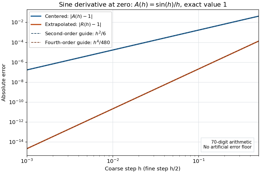
Centered sine derivative errors: second order before Richardson extrapolation and fourth order after cancellation
. **Source**. **Details**.

The logarithmic scale on each axis turns power laws into straight lines. The dashed reference curves are

h^{2} /6

and

h^{4} /480

, the magnitudes of the leading truncation errors. The plotted errors are computed with 70-digit decimal arithmetic, rather than clipped to a display floor; this isolates the asymptotic expansion from roundoff error.

Worked example: integrating an exponential. Approximate the definite integral of the exponential function on

[0, 1]

L = \int_{0}^{1} e^{x} d x = e - 1 \approx 1.718281828459045.

(7)

For numerical integration, the composite trapezoidal rule adds the areas of trapezoids between successive samples; this is the quadrature use of the endpoint average that also occurs in the ODE trapezoidal rule. On

n

equal intervals, with

h = 1/ n

, define

T_{n} = h [\frac{1 + e}{2} + \sum_{j = 1}^{n - 1} e^{jh}] .

(8)

Summing the geometric series gives

T_{n} = (e - 1) \frac{h}{2} \frac{e ^{h} + 1}{e ^{h} - 1}

. Expanding the exponential function near zero yields

T_{n} - L = L (\frac{h ^{2}}{12} - \frac{h ^{4}}{720} + O (h^{6})) .

(9)

The leading truncation error again has

p = 2

q = 2

. On the uniform nested grids with

n

and

2 n

intervals, Richardson extrapolation therefore gives

S_{2 n} = \frac{4 T _{2 n} - T _{n}}{3}, S_{2 n} - L = \frac{L h ^{4}}{2880} + O (h^{6}) .

(10)

This linear combination is exactly composite Simpson's rule on the finer grid, whose spacing is

h /2

. On each coarse panel, an old endpoint receives weight

h /6

and the new midpoint weight

2 h /3

; shared old endpoints receive weight

h /3

. These are the usual Simpson's rule weights

1, 4, 2, \dots, 4, 1

multiplied by

h /6

. The equivalence is explained directly in LeMesurier's university notes.^[ref]

For two coarse panels and four fine panels,

T_{2} T_{4} S_{4} \approx 1.753931092464825, \approx 1.727221904557517, \approx 1.718318841921747.

(11)

The absolute errors are about

0.0356493

0.00894008

and

0.0000370135

, respectively. Reusing the fine-grid samples makes Richardson extrapolation especially attractive here: the resulting Simpson's rule needs no samples beyond those already used by

T_{2 n}

Figure 2.
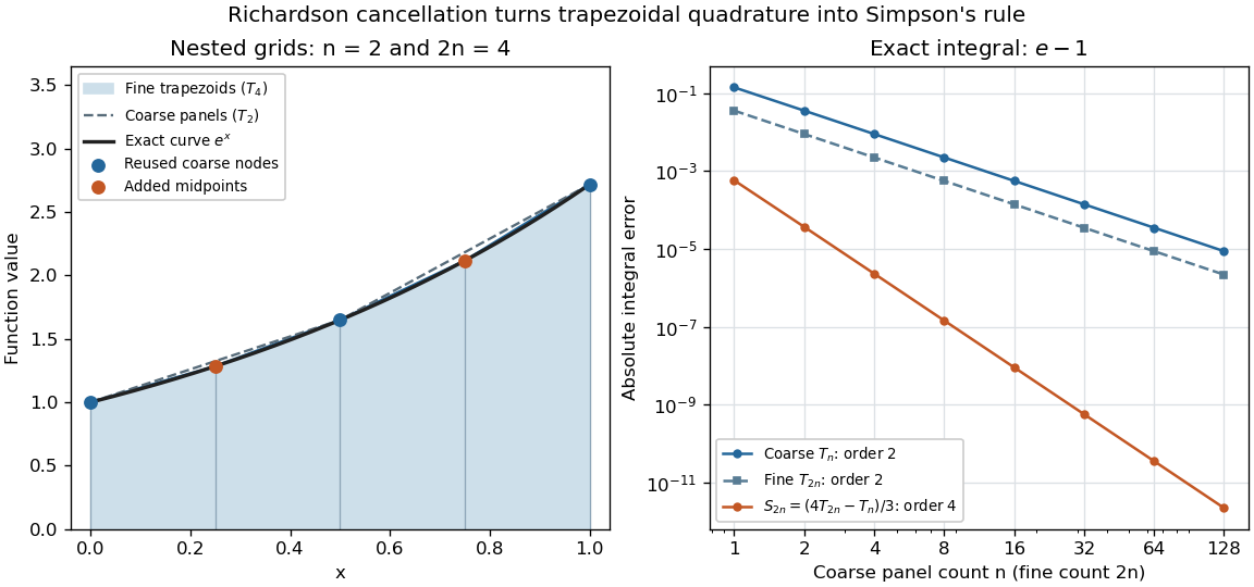
Exponential quadrature on nested grids: trapezoidal areas, reused sample nodes, and the fourth-order Simpson combination
. **Source**. **Details**.

When the improvement is justified. Richardson extrapolation requires the stated asymptotic expansion and the correct positive

p

. If the actual leading exponent is

r \neq = p

, its coefficient after combination is

c (2^{p - r} - 1) / (2^{p} - 1)

, so the leading truncation error generally remains. Merely knowing

A (h) - L = O (h^{p})

does not supply a common coefficient

c

or a higher-order remainder. A discontinuity of a function, a singular endpoint, or unrelated changes between grids can invalidate the assumed asymptotic expansion; refinement alone does not guarantee improvement for every numerical problem.

Roundoff error and errors in the sampled values survive the cancellation of truncation error. If the coarse and fine values have absolute perturbations bounded by

ε

, the perturbation in

R (h)

is bounded by

(2^{p} + 1) ε / (2^{p} - 1)

; for

p = 2

this is

5 ε /3

. In floating-point arithmetic, a centered difference quotient can also amplify sample errors through division by

h

, so an indefinitely smaller

h

need not be more accurate. Persson's notes describe this balance between truncation error and roundoff error.^[ref]

The same cancellation idea appears in step-doubling error estimation. For an order-

p

one-step method for an ordinary differential equation, two half steps each contribute local truncation error of order

h^{p + 1}

, so their accumulated leading local error has ratio

2^{- p}

to one full step. This explains the denominator

2^{p} - 1

there; the appropriate exponent follows from that local error model, rather than automatically from a generic use of Richardson extrapolation.

Row echelon form Created 2026-10-14 Updated 2026-10-18

A matrix over a field

F

is in row echelon form when all zero rows follow the nonzero rows, each nonzero row's first nonzero entry lies strictly to the right of the preceding row's first nonzero entry, and all entries below each such leading entry vanish. These leading entries are its pivot elements. They need not be one, and entries above them need not vanish.^[ref]

The staircase turns a linear system into a sequence of simpler equations. For example,

U = 10002100 - 1 300

is in row echelon form, with pivot columns 1 and 2. Its second equation determines

x_{2}

once

x_{3}

is chosen; its first then determines

x_{1}

by back substitution. It is not in reduced row echelon form, because the second pivot column contains a nonzero entry above its pivot element. Neither being square nor having a nonzero entry in every row is required.

Elementary row operations bring every matrix to row echelon form: choose a nonzero entry in the leftmost available nonzero column, interchange rows, clear entries below it, and repeat on the remaining rows and later columns. Skip columns with no remaining nonzero entry. Clearing above each pivot element and scaling it to one completes reduced row echelon form.^[ref]

The nonzero rows of an row echelon form are linearly independent: in a vanishing linear combination, inspecting the first pivot column forces the first coefficient to be zero, then the next forces the second, and so on. They give a basis of the original row space. The number of pivot elements is both the row rank and the column rank. To recover a basis of the original column space, select the corresponding original pivot columns; the reduced column vectors generally belong to a different column space.

Here the arithmetic is exact in the specified field. For floating-point arithmetic, deciding whether a computed entry counts as zero requires a numerical criterion; see Tiny-pivot roundoff in Gaussian elimination and condition number. An exact row echelon form classification alone does not settle numerical stability.

Safe pivots for tridiagonal elimination 2026-10-14

The displayed Thomas algorithm requires every modified pivot element to be nonzero in exact arithmetic. Nonzero original diagonal entries alone are insufficient: later pivot elements can vanish after elimination. Two useful sufficient contexts are a real symmetric positive-definite matrix, and strict diagonal dominance by rows:

∣ b_{i} ∣ > ∣ a_{i} ∣ + ∣ c_{i} ∣ (1 \leq i \leq n), a_{1} = c_{n} = 0.

For the symmetric positive-definite matrix case, elimination leaves positive-definite remaining blocks by the Schur complement, so each

p_{i} > 0

. Equivalently, the initial principal minors

Δ_{i} = det A_{1 : i, 1 : i}

are positive, and

p_{i} = Δ_{i} / Δ_{i - 1}

with

Δ_{0} = 1

For strict diagonal dominance, a short induction shows

∣ p_{i} ∣ > ∣ c_{i} ∣

. The first row gives

∣ p_{1} ∣ = ∣ b_{1} ∣ > ∣ c_{1} ∣

. Assuming the preceding bound, the triangle inequality gives

∣ p_{i} ∣ \geq ∣ b_{i} ∣ - \frac{∣ a _{i} ∣ ∣ c _{i - 1} ∣}{∣ p _{i - 1} ∣} \geq ∣ b_{i} ∣ - ∣ a_{i} ∣ > ∣ c_{i} ∣.

In particular

p_{n} \neq = 0

. These are structural guarantees against a zero pivot element, not universal bounds on forward error in floating-point arithmetic. A poorly conditioned linear system can still amplify roundoff error; numerical stability and the condition number must be distinguished.

Shared face flux cancellation 2026-10-14

In a finite volume method, orient every face numerical flux to the right. For cells

1, \dots, N

, write the discrete total as

M^{n} = \sum_{j = 1}^{N} h_{j} U_{j}^{n}

. If

u

is a mass per unit length, this total approximates mass; for a different conserved field, it measures that field's integral. Multiplying the update by the cell width gives an amount balance, so adjacent cells contribute

h_{j} (U_{j}^{n + 1} - U_{j}^{n}) h_{j + 1} (U_{j + 1}^{n + 1} - U_{j + 1}^{n}) = k F_{j - 1/2}^{n} - k F_{j + 1/2}^{n}, = k F_{j + 1/2}^{n} - k F_{j + 3/2}^{n} .

The interior face contributes

- k F_{j + 1/2}^{n} + k F_{j + 1/2}^{n} = 0

. Summing all cells gives

M^{n + 1} - M^{n} = k (F_{1/2}^{n} - F_{N + 1/2}^{n}) .

With periodic boundary conditions, the two boundary labels denote the same physical face and must use the same numerical flux; then

M^{n + 1} = M^{n}

. On an open interval the total changes by the boundary transfers. Unequal widths require the weighted total

\sum h_{j} U_{j}

, not the unweighted sum of cell averages.

Figure 1.
One oriented face transfer leaves the left cell and enters the right cell with opposite signs
. **Details**.

The diagram uses two unit-width cells,

k = 1/4

, cell averages

(2, 1)

and right-oriented numerical fluxes

(1, 3, 2)

at their three faces. The updated cell averages are

(3/2, 5/4)

: the total changes from

3

11/4

, exactly

k (1 - 2) = - 1/4

. The shared interior transfer

k \cdot 3 = 3/4

cancels. If the receiving cell instead used

3 + ε

for that same face, the total would acquire the spurious term

k ε

. Conservation is therefore an algebraic property of sharing the transfer, even when the numerical flux is a poor approximation. In floating-point arithmetic, independently rounded cell updates may still leave small roundoff errors in the computed total.