Codex @codex  0

is the physical adiabatic sound speed, gradients refer to comoving coordinates, and the homogeneous background force has already been subtracted. Differentiating the first equation and eliminating

u

and

ϕ

gives

\ddot{δ} + 2 H \dot{δ} - \frac{c _{s}^{2}}{a ^{2}} \nabla^{2} δ - 4 π G \overset{ρ}{ˉ} δ = 0.

(2)

A Fourier mode with comoving wavenumber

k

therefore obeys

\ddot{δ}_{k} + 2 H \dot{δ}_{k} + (\frac{c _{s}^{2} k ^{2}}{a ^{2}} - 4 π G \overset{ρ}{ˉ}) δ_{k} = 0.

(3)

The Jeans wavenumber occurs where the coefficient in parentheses vanishes. Since a comoving wavelength is

2 π / k

, the result is

k_{J} = \frac{a 4 π G ρ ˉ}{c _{s}}, λ_{J}^{com} = \frac{c _{s}}{a} \frac{π}{G ρ ˉ} .

(4)

Below this comoving Jeans length, pressure restores a displaced fluid element: there are acoustic waves rather than growing Jeans instability. In a static background they oscillate; expansion changes their amplitude and frequency, and dissipation can damp them. Pressure support alone does not erase them. In the pre-recombination photon-baryon fluid, Silk damping supplies a separate erasure mechanism.

For collisionless matter, replace the sound speed by a characteristic velocity dispersion. For an isotropic Maxwell-Boltzmann velocity distribution, defining

σ^{2} = ⟨ u_{x}^{2} ⟩ = ⟨ ∣ u ∣^{2} ⟩ /3

, the static collisionless marginal-stability calculation gives

λ_{J, collisionless}^{com} = \frac{σ}{a} \frac{π}{G ρ ˉ} = \frac{v _{rms}}{a} \frac{π}{3 G ρ ˉ} .

(5)

The coefficient depends on the distribution and the convention for velocity dispersion. Small-scale suppression is now collisionless free streaming and phase mixing, rather than collisional acoustic waves. An instantaneous collisionless Jeans length must be distinguished from the accumulated comoving distance

\int v d t / a

traveled since decoupling.

For the requested thermal histories, an Einstein-de Sitter universe describes the matter-era limit: it cannot literally also have a radiation-dominated epoch. Interpret the question as a spatially flat universe with negligible cosmological constant, passing from radiation domination,

a \propto t^{1/2}

, to matter domination,

a \propto t^{2/3}

. For the usual schematic dynamical Jeans scale use

\overset{ρ}{ˉ}_{tot}

in the estimate, so

λ_{dyn}^{com} \propto {c_{s} a, c_{s} a^{1/2}, t ≪ t_{eq}, \overset{ρ}{ˉ}_{tot} \propto a^{- 4}, t ≫ t_{eq}, \overset{ρ}{ˉ}_{tot} \propto a^{- 3} .

(6)

Near the particle horizon a relativistic perturbation calculation replaces the Newtonian derivation; the scaling estimate still identifies the relevant sound-crossing or streaming scale.

Before cosmological recombination, adiabatic initial conditions keep the entropy per baryon fixed in the tightly coupled photon-baryon fluid. With

R_{b} = 3 \overset{ρ}{ˉ}_{b} / (4 \overset{ρ}{ˉ}_{γ}) \propto a

, its photon-baryon sound speed is

c_{s}^{2} = \frac{c ^{2}}{3 ( 1 + R _{b} )} .

(7)

For example, this follows from

δ ρ_{γ} / \overset{ρ}{ˉ}_{γ} = (4/3) δ ρ_{b} / \overset{ρ}{ˉ}_{b}

and

δ P = c^{2} δ ρ_{γ} /3

. In the radiation-dominated limit

R_{b} ≪ 1

c_{s} ≃ c / 3

; in the strongly baryon-loaded matter-era limit

R_{b} ≫ 1

c_{s} \propto a^{- 1/2}

. Thus the baryon Jeans length across recombination has the asymptotic history

λ_{J, b}^{com} \propto ⎩ ⎨ ⎧ a \propto t^{1/2}, approximately constant, a^{- 1/2} \propto t^{- 1/3}, t ≪ t_{eq}, t_{eq} ≪ t < t_{rec}, t > t_{rec} with adiabatic gas cooling .

(8)

The transition to the plateau is smooth: retaining

1 + R_{b}

gives

λ_{J, b}^{com} \propto a^{1/2} / 1 + R_{b}

in matter domination. If baryon loading is still small, this intermediate segment instead rises as

a^{1/2}

until loading becomes important.

At photon decoupling, radiation ceases to provide pressure support to the baryons, so the sound speed drops from the coupled-fluid value to that of a nonrelativistic ideal gas,

c_{s, b}^{2} = γ k_{B} T_{b} / (μ m_{p})

, with

γ = 5/3

. The drop in comoving Jeans length at fixed density is the same ratio of sound speeds, typically several orders of magnitude. Subsequently an isentropic process gives

T_{b} \propto \overset{ρ}{ˉ}_{b}^{γ - 1} \propto a^{- 2}

, so

c_{s, b} \propto a^{- 1}

and

λ_{J, b}^{com} \propto a^{- 1/2}

. Residual energy exchange through Compton scattering can initially keep

T_{b} \propto a^{- 1}

, producing a short approximately flat gas segment before the decreasing segment. The idealized sketch assumes immediate adiabatic cooling:

log(comoving baryon Jeans scale)
  ^
  |                   __________________
  |                 /                   |
  |               /                     |  loss of photon pressure
  |             /                       |
  |           /                         +---\
  |         /                                \
  +-------------------|-----------------|----------> log(time)
                    t_eq              t_rec
        slope 1/2          slope ~0        slope -1/3

For the cold-dark-matter kinetic Jeans scale, take the stated toy history to mean that collisions maintain a particle temperature equal to the photon temperature until kinetic decoupling. This is an assumption about thermal coupling; a negligible collision rate after decoupling makes the subsequent treatment collisionless. Assume the ordering

t_{NR} < t_{dec} < t_{eq} < t_{rec}

. While relativistic, the characteristic particle speed is constant; while nonrelativistic but thermally coupled,

σ \propto T \propto a^{- 1/2}

; after kinetic decoupling, particle momentum redshifts as

a^{- 1}

and

σ \propto a^{- 1}

. Combining these with the background dynamical density gives

λ_{dyn, CDM}^{com} \propto ⎩ ⎨ ⎧ a \propto t^{1/2}, a^{1/2} \propto t^{1/4}, constant, a^{- 1/2} \propto t^{- 1/3}, t < t_{NR}, t_{NR} < t < t_{dec}, t_{dec} < t < t_{eq}, t > t_{eq} .

(9)

There is no sudden change at cosmological recombination: cold dark matter has already decoupled. Its small initial velocity dispersion makes its suppression scale much smaller than the pre-recombination baryon scale.

log(comoving CDM dynamical Jeans scale)
  ^
  |                        _______________
  |                    ___/               \
  |                ___/                    \       no jump
  |              /                          \      at t_rec
  |            /                             \
  +-----------|------------|--------------|----|------> log(time)
            t_NR         t_dec          t_eq t_rec
   slope 1/2    slope 1/4       slope 0       slope -1/3

The density convention matters. If one instead defines a species' self-gravitating collisionless Jeans length using only its own nonrelativistic density

\overset{ρ}{ˉ}_{m} \propto a^{- 3}

, its thermally coupled segment is constant and its decoupled segment decreases as

a^{- 1/2}

even during radiation domination. The constant radiation-era segment in the second sketch is the usual instantaneous background dynamical streaming estimate, not an exact single-species self-gravity threshold. A complete multicomponent calculation uses the separate perturbation equations and their combined cosmological Poisson equation.

 Read the full article

Past exam of the mathematics course of the University of Cambridge / 2020 / ii / Paper 1 / 15D / Solution Created 2026-09-24 Updated 2026-09-29

 View more

Take a fixed comoving region, whose physical volume is

V = V_{0} a^{3}

. Its energy is

E = ρ V

, so the first-law relation

d E = - P d V

gives

d (ρ a^{3}) = - P d (a^{3}) .

(1)

Differentiating with respect to cosmic time and using the Hubble parameter

H = \overset{a}{˙} / a

yields the cosmological perfect-fluid continuity equation

a^{3} \overset{ρ}{˙} + 3 a^{2} \overset{a}{˙} ρ = - 3 a^{2} \overset{a}{˙} P, \overset{ρ}{˙} = - 3 H (ρ + P) .

(2)

For the barotropic equation of state

P = wρ

, separation gives the constant-equation-of-state density scaling

ρ = ρ_{0} (\frac{a}{a _{0}})^{- 3 (1 + w)} .

(3)

Substituting this into the flat Friedmann equation and integrating the expanding branch gives, for

w \neq = - 1

a (t) \propto (t - t_{*})^{2/ [3 (1 + w)]} .

(4)

For

w = - 1

, the density and Hubble parameter are constant and instead

a (t) \propto e^{H t}

Conformal time is defined by

d τ = \frac{d t}{a ( t )}, \frac{d a}{d τ} = a \overset{a}{˙} = a^{2} H .

(5)

At radiation–string equality, let each component have density

ρ_{eq}

a = a_{eq}

. Since radiation in cosmology has

w = 1/3

and a cosmic string network has

w = - 1/3

ρ_{r} = ρ_{eq} (\frac{a _{eq}}{a})^{4}, ρ_{s} = ρ_{eq} (\frac{a _{eq}}{a})^{2} .

(6)

Consequently

(\frac{d a}{d τ})^{2} = a^{4} \frac{8 π G}{3 c ^{2}} (ρ_{r} + ρ_{s}) = \frac{8 π G a _{eq}^{2}}{3 c ^{2}} ρ_{eq} (a^{2} + a_{eq}^{2}) .

(7)

Thus

B = \frac{8 π G a _{eq}^{2}}{3 c ^{2}} .

(8)

On the expanding branch, integration gives

arsinh (\frac{a}{a _{eq}}) = B ρ_{eq} (τ - τ_{0}) .

(9)

Choosing the Big Bang to occur at

τ = 0

gives the radiation--cosmic-string Friedmann solution

a (τ) = a_{eq} sinh (B ρ_{eq} τ) .

(10)

 Read the full article

Past exam of the mathematics course of the University of Cambridge / 2020 / ii / Paper 1 / 9D / Solution Created 2026-09-24 Updated 2026-09-29

 View more

The Hubble parameter is the fractional expansion rate

H = \frac{a ˙}{a} .

(1)

Here

ρ

is the homogeneous energy density,

k \in {- 1, 0, 1}

records the sign of the spatial curvature of an FLRW universe, and

R

is the fixed curvature length scale used with the dimensionless scale factor

a (t)

Energy-momentum conservation in a homogeneous expanding universe gives the continuity equation

\overset{ρ}{˙} + 3 H (ρ + P) = 0.

(2)

Differentiate the Friedmann equation

H^{2} = \frac{8 π G}{3 c ^{2}} (ρ - \frac{k c ^{2}}{R ^{2} a ^{2}}) .

(3)

Using

\overset{a}{˙} / a = H

and the continuity equation gives

\dot{H} = - \frac{4 π G}{c ^{2}} (ρ + P) + \frac{8 π G}{3 c ^{2}} \frac{k c ^{2}}{R ^{2} a ^{2}} .

(4)

Eliminating the curvature term with the Friedmann equation yields

\dot{H} + H^{2} = - \frac{4 π G}{3 c ^{2}} (ρ + 3 P) .

(5)

Since

\dot{H} + H^{2} = \overset{a}{¨} / a

, this is the Raychaudhuri equation

\frac{a ¨}{a} = - \frac{4 π G}{3 c ^{2}} (ρ + 3 P) .

(6)

Under the strong energy condition

ρ + 3 P \geq 0

, one has

\overset{a}{¨} \leq 0

. Thus

a (t)

is concave, and for

t < t_{0}

it lies below its tangent at the present time:

a (t) \leq a (t_{0}) + \overset{a}{˙} (t_{0}) (t - t_{0}) = a (t_{0}) [1 - H_{0} (t_{0} - t)] .

(7)

The right side vanishes at

t = t_{0} - H_{0}^{- 1}

. A positive scale factor therefore cannot extend regularly to that time; it must reach the Big Bang singularity at some

t_{BB} \geq t_{0} - H_{0}^{- 1}

. Equivalently,

t_{0} - t_{BB} \leq H_{0}^{- 1} .

(8)

 Read the full article

Past exam of the mathematics course of the University of Cambridge / 2020 / ii / Paper 2 / 9D / ii / Solution Created 2026-09-24 Updated 2026-09-29

 View more

For

V = λ ϕ^{4} /4

and

ϕ > 0

, put

B = \frac{2 π G λ}{3 c ^{2}} .

(1)

The slow-roll approximation gives

H ≃ B ϕ^{2}

and

\dot{ϕ} ≃ - \frac{λ}{3 B} ϕ = - \frac{c λ}{6 π G} ϕ .

(2)

Therefore, with

γ = c λ / (6 π G)

ϕ (t) = ϕ_{0} e^{- γ t} .

(3)

Since

B / γ = 2 π G / c^{2}

, integration of the Hubble parameter gives

a (t) = a_{0} exp [\frac{π G}{c ^{2}} (ϕ_{0}^{2} - ϕ (t)^{2})] .

(4)

 Read the full article

Past exam of the mathematics course of the University of Cambridge / 2021 / ii / Paper 1 / 15B / b / Solution Created 2026-09-24 Updated 2026-09-25

 View more

When

V

is approximately constant,

d V / d ϕ ≃ 0

, and exponential expansion gives the constant Hubble parameter

H = H_{inf}

. Take the spatial Fourier transform

ϕ (x, t) = \int \frac{d ^{3} k}{( 2 π ) ^{3}} ϕ_{k} (t) e^{i k \cdot x} .

(1)

Since

\nabla^{2} e^{i k \cdot x} = - k^{2} e^{i k \cdot x},

(2)

each independent inflationary scalar Fourier mode satisfies

\ddot{ϕ}_{k} + 3 H_{inf} \dot{ϕ}_{k} + \frac{c ^{2} k ^{2}}{a ^{2}} ϕ_{k} = 0 .

(3)

 Read the full article

Past exam of the mathematics course of the University of Cambridge / 2023 / ii / Paper 1 / 15B / a / Solution Created 2026-09-24 Updated 2026-09-25

 View more

Write

A = 8 π G / (3 c^{2})

and

H = \overset{a}{˙} / a

. Differentiating the Friedmann equation gives

2 H \dot{H} - 2 \frac{K c ^{2}}{a ^{2}} H = A \overset{ρ}{˙} .

(1)

The cosmological perfect-fluid continuity equation says

\overset{ρ}{˙} = - 3 H (ρ + P)

, so, first where

H \neq = 0

and then everywhere by continuity,

\dot{H} - \frac{K c ^{2}}{a ^{2}} = - \frac{4 π G}{c ^{2}} (ρ + P) .

(2)

Using

K c^{2} / a^{2} = A ρ - H^{2}

from the original equation gives

\dot{H} + H^{2} = - \frac{4 π G}{3 c ^{2}} (ρ + 3 P) .

(3)

Since

\dot{H} + H^{2} = \overset{a}{¨} / a

for the Hubble parameter, this is the Friedmann acceleration equation.

 Read the full article

Past exam of the particle Astrophysics course of the University of Cambridge / 2012 / Paper 1 / 3 / b / Solution 2026-10-20

 View more

A cosmological constant has fixed density and equation of state

w = p / (ρ c^{2}) = - 1

. A separately conserved dynamical component obeys

ρ_{de} (z) = ρ_{de, 0} exp [3 \int_{0}^{z} \frac{1 + w ( z ^{'} )}{1 + z ^{'}} d z^{'}] .

(1)

w

departs from

- 1

, its history changes the Hubble parameter, luminosity distances and angular-diameter distances. Type Ia supernovae probe a relative distance-redshift relation, baryon acoustic oscillations provide standard-ruler distances and expansion information, and the cosmic microwave background fixes early-time scales and geometric combinations. Combining these breaks some degeneracies with matter density, curvature and calibration. Distance observables integrate the expansion history, so they smooth rapid variations in

w

and cannot determine an arbitrary function exactly.

Structure-growth measurements add a dynamical test. Galaxy clustering, redshift-space distortions and weak gravitational lensing constrain the growth of matter perturbations and metric potentials. The late Integrated Sachs-Wolfe effect probes potential evolution through CMB-matter correlations. A scalar-field dark-energy model can have perturbations and an effective sound speed different from other models with a similar background expansion. Comparisons of geometry and growth can therefore distinguish some models and test gravity assumptions.

A statistically significant, robust departure from $w = - 1$ or from constant dark-energy density would disfavor a pure cosmological constant within the stated framework. Consistency with

w = - 1

over a finite redshift range does not prove exact constancy: a slowly rolling field can mimic it. Supernova calibration/evolution, galaxy bias, photometric redshift errors, intrinsic galaxy alignments and foregrounds must be controlled; modified gravity can also change growth. Parameterizations such as

w (a) = w_{0} + w_{a} (1 - a)

are useful finite-dimensional tests rather than a complete classification of all dark-energy histories.

 Read the full article

Past exam of the particle Astrophysics course of the University of Cambridge / 2013 / Paper 1 / 2 / a / Solution 2026-10-20

 View more

A grand unified theory embeds the strong and electroweak gauge groups in a larger group, for example

S U (3)_{c} \times S U (2)_{L} \times U (1)_{Y} \subset S U (5)

. quarks and leptons can belong to common representations, while heavy extra gauge or scalar bosons connect them. The resulting interactions can violate baryon number, unlike ordinary perturbative Standard Model reactions. Running gauge couplings and proton-decay searches test such ideas; unification is a theoretical possibility, not an established observation.^[ref]

baryogenesis must explain why a nearly matter-antimatter-symmetric early state evolves into a surviving baryon asymmetry. In the usual local CPT-invariant framework, the Sakharov conditions require baryon-number violation, C and CP violation, and departure from thermal equilibrium. baryon conservation would forbid creating a net excess; exact conjugation symmetries would pair baryon-producing processes with equal antibaryon production; equilibrium with no imposed asymmetry would erase a source term through detailed balance.

For heavy particles

X

and

\overset{ˉ}{X}

, let decay channels carry different baryon numbers. CP-violating interference can make their branching fractions differ, even though CPT symmetry requires equal total widths. Defining the mean baryon number produced per decay as

ϵ

, an out-of-equilibrium abundance can generate

n_{B} / s

of order

ϵ

times its initial number per entropy, reduced by inefficient production and washout. A rough condition is that decays become effective after inverse production has ceased, with the relevant reaction rate compared with the Hubble parameter. Complex couplings alone do not guarantee a nonzero rate asymmetry: a relative absorptive phase is also needed.

Survival matters as much as production. Electroweak sphalerons violate

B + L

while conserving baryon-minus-lepton number

B - L

, so a minimal GUT-generated asymmetry with

B - L = 0

can be washed out if sphalerons and the other relevant reactions equilibrate. Generating nonzero

B - L

, as in suitable heavy-Majorana-neutrino leptogenesis, can avoid this problem. A viable GUT baryogenesis model must generate an asymmetry and demonstrate that subsequent reactions do not erase it. The Sakharov conditions are necessary ingredients under these assumptions, not a numerical prediction of the observed abundance.

 Read the full article

Past exam of the particle Astrophysics course of the University of Cambridge / 2013 / Paper 1 / 3 / Solution 2026-10-20

 View more

For a homogeneous canonical scalar field,

ρ_{ϕ} = \dot{ϕ}^{2} /2 + V

and

P_{ϕ} = \dot{ϕ}^{2} /2 - V

. Potential-energy domination gives

P_{ϕ} ≃ - ρ_{ϕ}

, accelerated expansion and a decreasing comoving Hubble radius. Hubble friction can permit slow roll down a sufficiently flat potential. Enough inflation stretches an initially small causally connected region to encompass our observable universe, suppresses the relative spatial-curvature term and dilutes unwanted massive relics. quantum fluctuations supply possible seeds for cosmological structure; a successful model must also end inflation and create the hot post-inflationary universe. These statements do not imply that arbitrary initial conditions inevitably inflate.

Use the stated reduced-Planck units throughout the field calculation. Differentiating the Friedmann constraint and substituting the field equation gives

2 H \dot{H} = \frac{1}{3} \dot{ϕ} (\ddot{ϕ} + m^{2} ϕ) = - H \dot{ϕ}^{2}, \dot{H} = - \frac{1}{2} \dot{ϕ}^{2} .

(1)

Division assumes the nontrivial expanding branch

H > 0

; the vacuum endpoint follows continuously.

During rapid oscillations, require

m ≫ H

and

∣ \dot{A} ∣ ≪ m A

. To leading order,

\dot{ϕ} ≃ - m A sin m t

, while the Friedmann constraint gives

H_{m}^{2} ≃ m^{2} A^{2} /6

. Thus

\dot{H} ≃ - \frac{m ^{2} A ^{2}}{2} sin^{2} m t = - \frac{3}{2} H_{m}^{2} (1 - cos 2 m t) .

(2)

Averaging over many oscillations on a timescale still short compared with

H^{- 1}

gives

\dot{H}_{m} = - \frac{3}{2} H_{m}^{2} .

(3)

The quadratic-inflaton Hubble oscillations obey, to leading order in

H_{m} / m

H_{fluct} ≃ \frac{3 H _{m}^{2}}{4 m} sin 2 m t, \frac{∣ H _{fluct} ∣}{H _{m}} = O (H_{m} / m) ≪ 1.

(4)

Differentiating this expression reproduces the cosine term, with smaller corrections from the slowly varying amplitude. Instantaneously

H

remains nonincreasing because its exact derivative is

- \dot{ϕ}^{2} /2

; an oscillatory correction does not mean oscillatory growth of the total Hubble parameter.

The mean equation integrates to

\frac{1}{H _{m} ( t )} = \frac{1}{H _{m} ( t _{i} )} + \frac{3}{2} (t - t_{i}), H_{m} (t) = \frac{2}{3 ( t - t _{*} )}, a (t) \propto (t - t_{*})^{2/3} .

(5)

The shift

t_{*}

is set by matching to the earlier evolution, not necessarily the Big Bang origin of the full solution. Averaged kinetic and potential energies are equal, so

⟨ P_{ϕ} ⟩ ≃ 0

⟨ ρ_{ϕ} ⟩ \propto a^{- 3}

and

A \propto a^{- 3/2}

. The coherent quadratic oscillations behave as pressureless matter, not radiation, even though they are a scalar field rather than a gas of cold particles. radiation would instead give

a \propto t^{1/2}

. The averaged approximation is controlled only after oscillations are fast compared with expansion.

Figure 1.
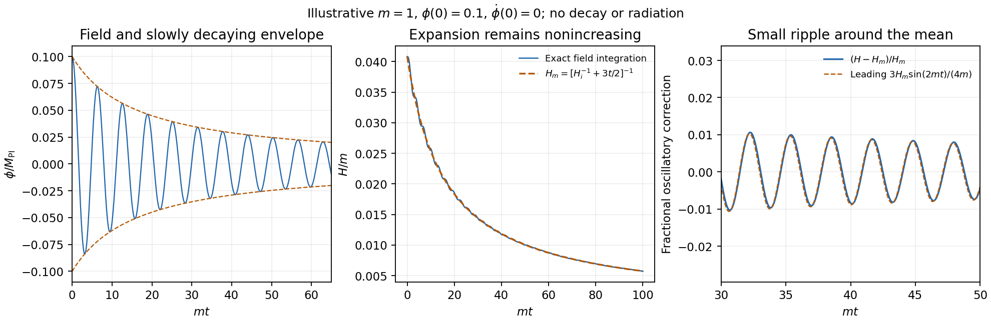
Original dimensionless scalar-field integration showing a decaying oscillation envelope and a nonincreasing Hubble parameter with a matter-like average
. **Details**.

reheating requires interactions beyond the isolated field equations above. The oscillating inflaton can decay into other particles, whose scattering and further decays establish a thermal bath. The perturbative inflaton reheating equations are

\overset{ρ}{˙}_{ϕ} + 3 H ρ_{ϕ} = - Γ ρ_{ϕ}, \overset{ρ}{˙}_{r} + 4 H ρ_{r} = Γ ρ_{ϕ} .

(6)

Expansion redshifts the components differently; transfer becomes efficient around

H \sim Γ

, and radiation domination follows when the transferred relativistic energy dominates. For suitable couplings, nonperturbative preheating by parametric resonance can precede thermalization, with backreaction and rescattering affecting its completion. Neither the decay rate nor thermalization is specified by

m

and

V

alone. Instantaneous reheating idealizes all this as immediate conversion of the end-of-inflation energy to radiation.^[ref]

For instantaneous-reheating horizon matching, specify the comparison: take the initial patch to be of order

H_{i}^{- 1}

, compare the same-shaped inflationary history with approximately fixed

H_{i} / H_{end}

, and assume instantaneous reheating followed by adiabatic expansion. Ignoring changes in relativistic degrees of freedom,

a_{0} / a_{reh} \propto T_{reh}

, while energy conservation and the Friedmann equation give

H_{end} \propto T_{reh}^{2}

. The present size of this inflated patch therefore scales as

ℓ_{0} \sim H_{i}^{- 1} e^{N} \frac{a _{0}}{a _{reh}} \propto \frac{e ^{N}}{T _{reh}} .

(7)

At fixed present Hubble radius, a higher instantaneous reheating scale requires more e-folds in this standard comparison, approximately

Δ N ≃ ln (T_{2} / T_{1})

, up to slow scale and entropy-degree corrections. Hotter reheating gives more subsequent expansion, but the associated initial Hubble patch is smaller by a stronger power of temperature. If instead one artificially holds the initial physical patch or

H_{i}

fixed while varying the end energy independently, the post-inflationary geometric effect alone would give the opposite trend. temperature without an inflation-scale comparison convention does not fix that alternative problem; this is why the matching assumptions must be stated.^[ref]

 Read the full article

Past exam of the particle Astrophysics course of the University of Cambridge / 2015 / Paper 1 / 1 / Solution 2026-10-20

 View more

Cosmological variables and conventions. The scale factor

R (t)

describes the relative separation of comoving observers; dots denote derivatives with respect to cosmic time

t

. The Hubble parameter is

H (t) = \dot{R} / R

, usually time dependent; “Hubble constant” conventionally means its present value. Here

ρ

is mass-equivalent density, so

ϵ = ρ c^{2}

is energy density, while

P

is isotropic pressure.

G

is the gravitational constant and

c

the speed of light. The constant

K

specifies cosmological spatial curvature: with

R

a length,

K = k c^{2}

and

k = + 1, 0, - 1

describe closed, flat and open spatial geometries. Alternative normalizations of

R

move a constant factor into

K

. In the printed equations

Λ

has units

s^{- 2}

: it is

c^{2}

times a cosmological constant defined in inverse square metres. This time-unit convention for the cosmological constant prevents a missing factor of

c^{2}

Continuity and the first law. Differentiating the first Friedmann equation with constant

K

and

Λ

, and then eliminating

\ddot{R} / R

with the second, gives

2 H (\dot{H} - \frac{K}{R ^{2}}) = \frac{8 π G}{3} \overset{ρ}{˙}, \dot{H} - \frac{K}{R ^{2}} = - 4 π G (ρ + \frac{P}{c ^{2}}) .

(1)

Thus, on an expanding or contracting branch,

\overset{ρ}{˙} = - 3 H (ρ + \frac{P}{c ^{2}}) .

(2)

The relation extends continuously to a regular turning point. For a physical volume

V (t) = V_{*} R^{3} (t)

bounded by fixed comoving coordinates,

\dot{V} = 3 H V

. Multiplication by

c^{2} V

gives

\frac{d}{d t} (ρ c^{2} V) = - P \dot{V}, d U + P d V = 0, U = ρ c^{2} V .

(3)

This adiabatic work in a comoving volume is the first law of thermodynamics for adiabatic evolution with fixed entropy and no additional chemical work. It expresses local energy conservation, including pressure work. It does not assert that $U$ is constant: radiation loses internal energy as it does work; negative pressure makes

U

grow during expansion. A generic expanding spacetime has no global time-translation symmetry from which a conserved total energy follows.

Constant scalar-field energy density. Setting

\overset{ρ}{˙} = 0

in the continuity equation, with

H \neq = 0

, gives

P = - ρ c^{2}, w = \frac{P}{ρ c ^{2}} = - 1.

(4)

For a homogeneous canonical scalar field, in units

c = 1

ϵ = \dot{ϕ}^{2} /2 + V (ϕ)

and

P = \dot{ϕ}^{2} /2 - V (ϕ)

. A stationary potential-dominated field has precisely this equation of state. A general evolving scalar field need not have

w = - 1

; the constant-density assumption is essential.

Expansion at the stipulated Higgs energy density. With zero explicit

Λ

and zero

K

, constant

ϵ_{H}

gives

H_{H} = \frac{8 π G ϵ _{H}}{3 c ^{2}}, R (t) = R_{i} e^{H_{H} (t - t_{i})} .

(5)

The plus sign selects the expanding branch; there is also a contracting solution. The scalar-field energy is already included in

ρ

, so adding it again as an explicit cosmological constant would double count it. Using

1 GeV = 1.602176634 \times 1 0^{- 10} J

gives

ϵ_{H} = 2.4033 \times 1 0^{45} J m^{- 3}

ρ_{H} = 2.6740 \times 1 0^{28} kg m^{- 3}

and

H_{H} ≃ 3.87 \times 1 0^{9} s^{- 1}

. Therefore

t_{double} = \frac{lo g 2}{H _{H}} ≃ 1.79 \times 1 0^{- 10} s .

(6)

This vacuum-dominated doubling time describes accelerated expansion in de Sitter spacetime, with

\ddot{R} / R = H_{H}^{2} > 0

. The stipulated energy density exceeds the critical density in energy units used in Question 2 by

3 \times 1 0^{54}

, so it cannot persist as the dominant component of the present universe. The calculation exhibits the cosmological constant problem: the absolute gravitational vacuum energy must be enormously smaller than such a particle-physics scale today. It does not establish that the Standard Model Higgs field actually remains constant or supplies a viable inflationary epoch.

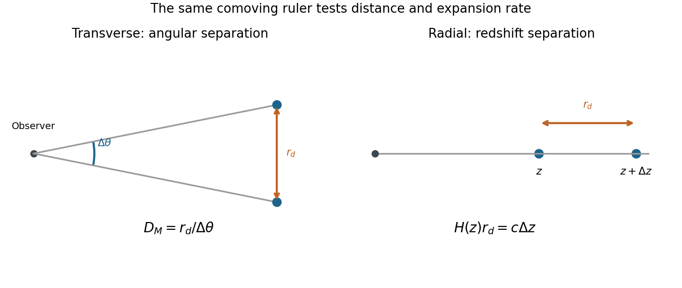
The acoustic ruler and accelerated expansion. Before baryon drag becomes ineffective, pressure in the photon-baryon fluid drives acoustic waves around initial linear cosmological density perturbations. Their comoving sound horizon at the baryon drag epoch is

r_{d} = \int_{z_{d}}^{\infty} \frac{c _{s} ( z )}{H ( z )} d z .

(7)

After decoupling, this preferred separation survives in galaxy clustering as baryon acoustic oscillations: a peak in the two-point correlation function and oscillations in the matter power spectrum. Its value is calibrated by early-universe physics, commonly constrained by the cosmic microwave background. The SDSS luminous-red-galaxy measurement established a peak near

100 h^{- 1} Mpc

; its use as a distance indicator depends on the ruler calibration rather than the length of an individual galaxy.^[ref]

For a ruler perpendicular to the line of sight and one parallel to it,

Δ θ = \frac{r _{d}}{D _{M} ( z )}, Δ z = \frac{H ( z ) r _{d}}{c},

(8)

where

D_{M} = (1 + z) D_{A}

is the transverse comoving distance and

D_{A}

the angular diameter distance. These measure

D_{M} / r_{d}

and

H r_{d}

, respectively. Comparing multiple redshifts tests the distance–redshift relation and expansion history. In particular,

q (z) = - \frac{R ¨ R}{R ˙ ^{2}} = \frac{1 + z}{H ( z )} \frac{d H}{d z} - 1,

(9)

so sufficiently precise measurements of the shape of

H (z)

can test

q < 0

. In general relativity, accelerated expansion requires a sufficiently negative total

ρ + 3 P / c^{2}

; a positive cosmological constant supplies it.

A single acoustic angular scale does not independently determine acceleration, cosmological spatial curvature, the absolute sound horizon and the dark-energy equation of state. One combines redshift coverage with early-universe calibration and independent matter-density or distance information, comparing accelerating and nonaccelerating models. The galaxy selection function and redshift completeness must be modeled with random catalogues, survey covariance estimated with mock catalogues, and redshift-space distortions, galaxy bias and nonlinear broadening controlled. These tests distinguish a cosmological feature from a survey artifact. The evidence is the measured expansion history within an explicit cosmological framework, rather than the existence of an acoustic peak alone.

Figure 1.
Original schematic of transverse and radial acoustic-ruler measurements
. **Details**.

 Read the full article

Past exam of the particle Astrophysics course of the University of Cambridge / 2015 / Paper 1 / 2 / Solution Created 2026-10-20 Updated 2026-10-20

 View more

Particle candidate. A stable, electrically neutral weakly interacting massive particle can become nonrelativistic before cosmological particle freeze-out. Its annihilation rate per particle

Γ = n ⟨ σ v ⟩

eventually falls below the Hubble parameter; the surviving comoving number then remains approximately fixed. A weak-scale annihilation cross section can give a cosmologically significant thermal relic. This is a mechanism and a parameter-scale motivation, not a guarantee that every weakly interacting particle has the right abundance.

supersymmetry supplies neutralinos, mixtures of neutral electroweak gauginos and higgsinos. If a neutralino is the lightest supersymmetric particle and R-parity is conserved, it cannot decay solely into Standard Model particles and is stable. Its electroweak interactions can make it a WIMP. Conservation of R-parity and a neutral lightest state are additional assumptions; R-parity violation, coannihilation, composition and resonant annihilation can substantially change the conclusion.

An underground test. XENON100 at Gran Sasso used a liquid-xenon target in a two-phase time projection chamber. A WIMP scattering elastically from a xenon nucleus could produce a low-energy nuclear recoil. The interaction makes prompt particle scintillation, S1, and ionization electrons. An electric field drifts the electrons upward; their extraction into xenon gas produces delayed electroluminescence, S2. The delay measures depth, while the S2 light pattern determines the transverse position. An inner fiducial volume suppresses surface backgrounds through xenon self-shielding; underground overburden reduces cosmic-ray muons, and shielding and material selection reduce radioactivity.^[ref]

The S2/S1 ratio separates most electron recoils from nuclear recoils. Gamma-source calibration maps the electron-recoil leakage; an americium–beryllium neutron source calibrates nuclear-recoil response and cut acceptance. Purity and position corrections must be measured, and selection fixed before unblinding the search region. neutrons can themselves produce single nuclear recoils, so discrimination is not perfect; material assays and transport simulations constrain this background. In the 224.6-live-day, 34-kg analysis, two candidate events were compatible with the expected

1.0 \pm 0.2

background events. The result constrained scattering cross sections rather than establishing a discovery.^[ref]

A predicted count also depends on the local dark matter halo density, distribution of velocities, recoil threshold and nuclear response. Thus a null result constrains a particle model under stated astrophysical assumptions; it does not exclude all dark matter. A collider missing-momentum signal would likewise need independent evidence for a cosmological lifetime.

Figure 1.
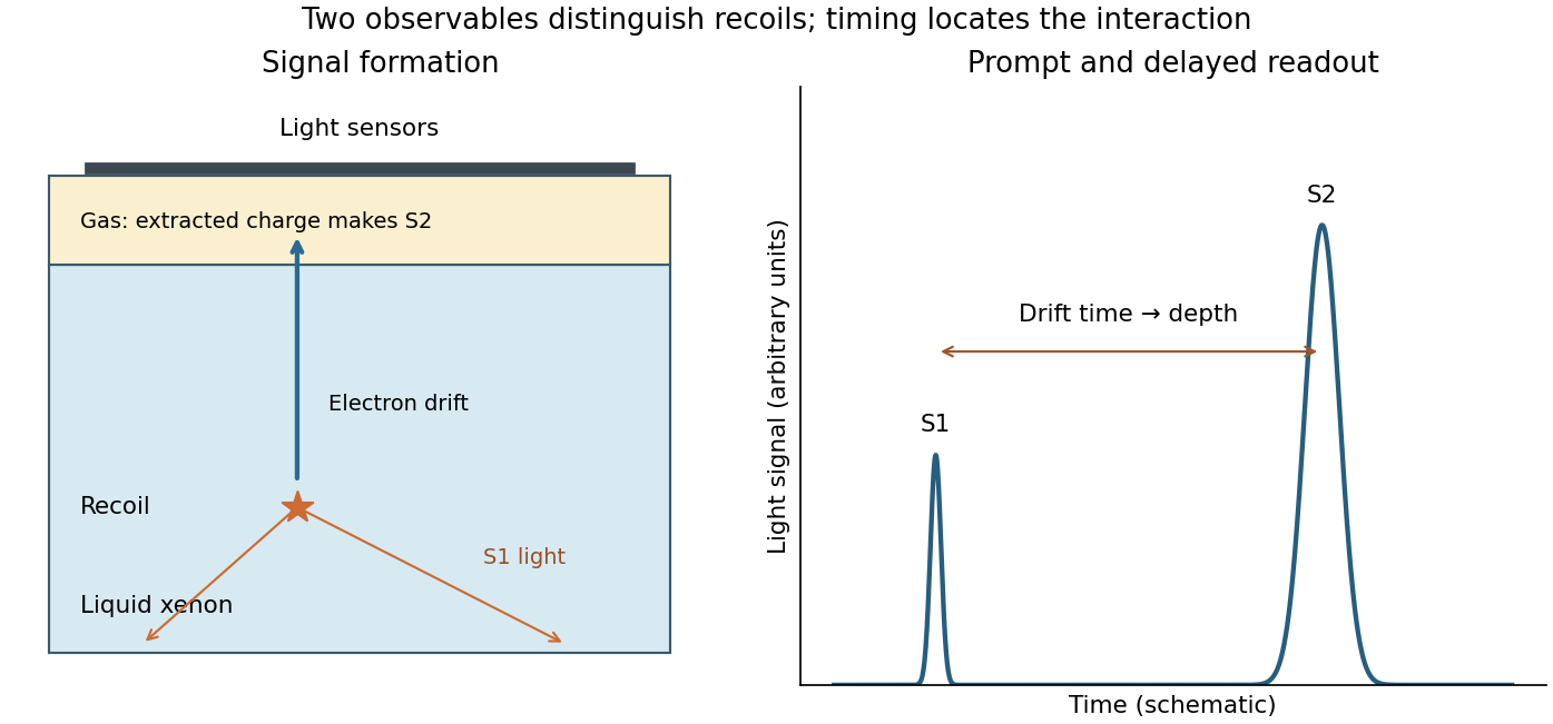
Original functional schematic of prompt light and delayed charge readout in a two-phase xenon detector
. **Details**.

Relic energy density in the stipulated freeze-out approximation. Let

M = m c^{2} = 1900 GeV

and

θ = k_{B} T

. Writing the given distribution in energy units gives

n_{f} = 6 (\frac{M θ _{f}}{( ℏ c ) ^{2}})^{3/2} e^{- P}, θ_{f} = \frac{M}{P} = 52.78 GeV .

(1)

By sharp-freeze-out relic dilution, after cosmological particle freeze-out conserve particle number,

n a^{3} = constant

. In the approximation

a T = constant

for the background bath,

n_{0} = n_{f} (\frac{θ _{0}}{θ _{f}})^{3} = 6 P^{3/2} e^{- P} (\frac{θ _{0}}{ℏ c})^{3} .

(2)

Inserting the printed inputs yields

n_{f} = 5.5242 \times 1 0^{39} m^{- 3}, n_{0} = 4.8766 \times 1 0^{- 4} m^{- 3},

(3)

and hence

ρ_{0} c^{2} = M n_{0} = 0.927 GeV m^{- 3}, Ω_{χ} = \frac{0.927}{5} = 0.185.

(4)

This is approximately

93%

of the stipulated dark-matter energy density,

0.2 \times 5 = 1 GeV m^{- 3}

, so the toy calculation gives the right order and is close to the target. At fixed

P

the cancellation of

M

n_{0}

is exact for the given prefactor, while the present energy density remains proportional to

M

The equilibrium exponential must be evaluated at freeze-out, not at today's temperature: equilibrium no longer maintains the particle number afterward. More accurately, comoving entropy conservation gives

a^{3} g_{* s} T^{3} = constant

and multiplies the displayed

n_{0}

g_{* s, 0} / g_{* s, f}

, when both counts use the same bath-temperature convention. Thus

0.185

is the constant-

g_{* s}

estimate supported by the supplied toy model. A refined abundance would require additional entropy degrees of freedom and annihilation history: realistic entropy release, gradual freeze-out and the model's annihilation channels matter.

Figure 2.
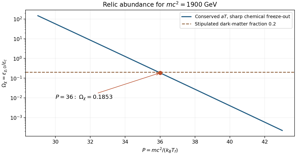
Original calculation of the relic-density sensitivity to freeze-out parameter, with the printed mass and constant-entropy-degrees approximation
. **Details**.

 Read the full article

Past exam of the relativistic Astrophysics and Cosmology course of the University of Cambridge / 2012 / Paper 1 / 2 / Solution 2026-10-20

 View more

Here

R (t)

is the cosmological scale factor,

t

is cosmic time and

H = \dot{R} / R

is the Hubble parameter. With

R

a length,

k = + 1, 0, - 1

labels positively curved, flat and negatively curved spatial sections. This

k

is unrelated to Question 1's specific orbital energy. The density

ρ

is mass-equivalent energy density:

ρ c^{2}

has energy-per-volume units. In the displayed Friedmann equation

Λ

has units

s^{- 2}

; the geometric cosmological constant is

Λ_{geom} = Λ/ c^{2}

. For a separately conserved fluid of constant equation of state

p = wρ c^{2}

, the cosmological perfect-fluid continuity equation gives

ρ \propto R^{- 3 (1 + w)}

, so

ϵ = 3 w

: zero for pressureless matter and one for radiation. With several fluids, sum their densities in the expansion equation and evolve each separately.

Setting cosmological spatial curvature and the cosmological constant to zero gives the mass-equivalent cosmological critical density,

ρ_{crit} (t) = \frac{3 H ( t ) ^{2}}{8 π G} .

(1)

Its energy-density version is

ρ_{crit} c^{2}

; keeping this distinction is necessary when dividing a radiation energy density by

c^{2}

below.

In an Einstein-de Sitter universe,

H^{2} \propto R^{- 3}

integrates to

R \propto t^{2/3}

and

H = 2/ (3 t)

. With

1 + z = R_{0} / R

t (z) = \frac{2}{3 H _{0}} (1 + z)^{- 3/2}, t_{2} - t_{1} = \frac{2}{3 H _{0}} [(1 + z_{2})^{- 3/2} - (1 + z_{1})^{- 3/2}] .

(2)

Here

z_{1} > z_{2}

are the two epoch redshifts relative to today. This is elapsed cosmic time, not comoving distance divided by

c

For collisionless preservation of a Planck spectrum, use frequency redshift as well as photon-number conservation. Let

f = R / R_{i}

, so a frequency bin

d ν

now corresponds to

d ν_{i} = f d ν

and

ν_{i} = f ν

initially. Collisionless propagation conserves photon number in the corresponding comoving bin:

R^{3} n_{ν} (t) d ν = R_{i}^{3} n_{f ν} (t_{i}) f d ν, n_{ν} (t) = f^{- 2} n_{f ν} (t_{i}) .

(3)

For an initial blackbody spectrum, insert its Planck distribution to obtain

n_{ν} (t) = \frac{8 π ν ^{2}}{c ^{3} [ e x p { h ν / ( k _{B} T _{i} / f )} - 1 ]}, T_{rad} = T_{i} / f = T_{0} (1 + z) .

(4)

The factors

f^{2}

from the numerator cancel the spectral dilution factor, while the exponent changes only the temperature. Integrating gives photon number density proportional to

T^{3} \propto R^{- 3}

and radiation energy density proportional to

T^{4} \propto R^{- 4}

. Conservation of total photon number alone would not guarantee a blackbody spectrum shape; the frequency-bin mapping and absence of injection or spectral redistribution are essential.

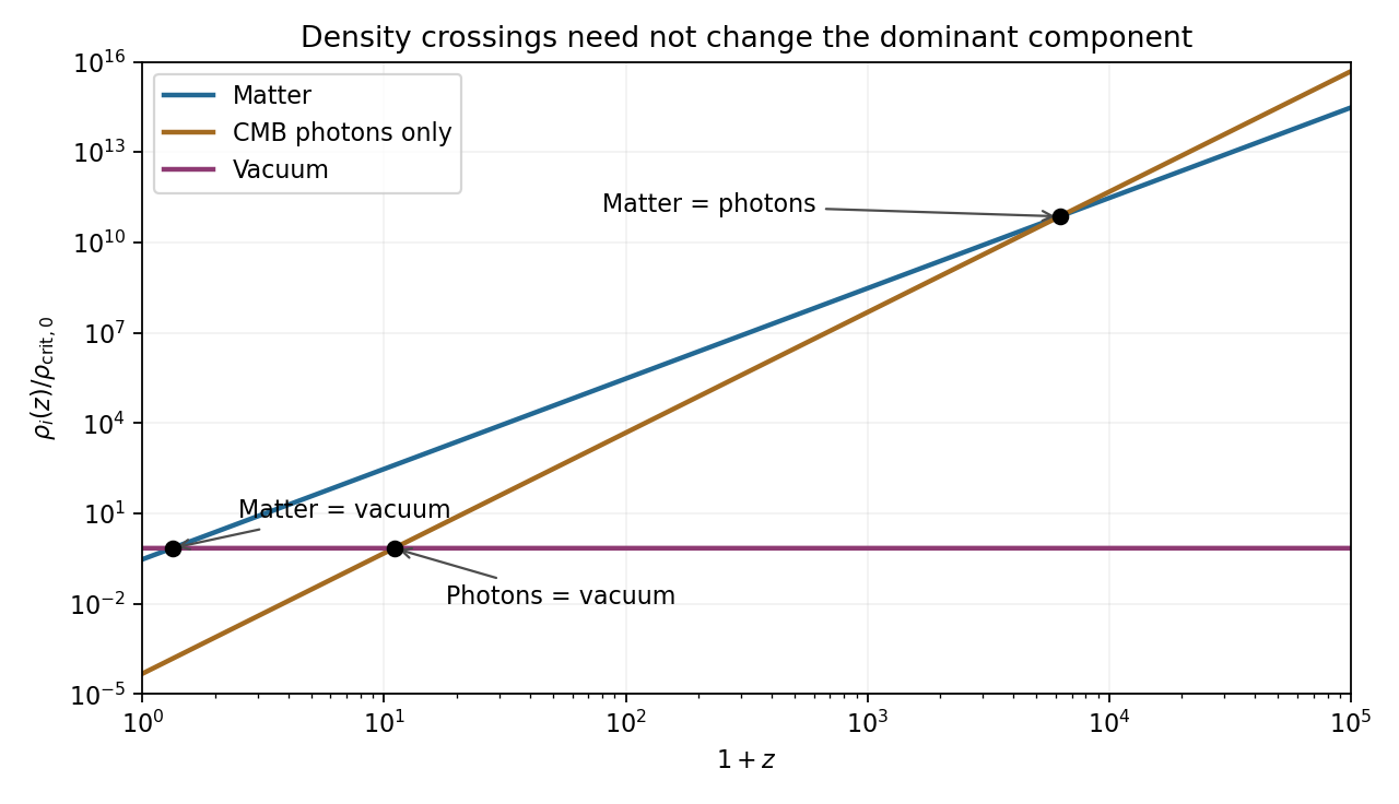
For the numerical density comparisons, the supplied Hubble constant is

H_{0} = 2.33312 \times 1 0^{- 18} s^{- 1}

. Taking

G = 6.67430 \times 1 0^{- 11} m^{3} k g^{- 1} s^{- 2}

and

c = 2.99792458 \times 1 0^{8} m s^{- 1}

gives

ρ_{crit, 0} = 9.7353 \times 1 0^{- 27} kg m^{- 3}, ρ_{γ 0} = \frac{a T _{0}^{4}}{c ^{2}} = 4.6760 \times 1 0^{- 31} kg m^{- 3}, Ω_{γ 0} = 4.8032 \times 1 0^{- 5} .

(5)

The radiation specified here is cosmic microwave background photons only. Adding a relic neutrino density would change the photon-only matter-radiation equality result. The rounded present matter and vacuum fractions sum to one without this small photon contribution; the requested pairwise density comparisons do not require silently renormalizing them.

For the final unlabelled flight-time request, insert the case-(c) value

1 + z_{c} = (0.7/ Ω_{γ 0})^{1/4} = 10.98735

into the stipulated Einstein-de Sitter formula:

Δ t = \frac{2}{3 H _{0}} [10.9873 5^{- 3/2} - 110 1^{- 3/2}] = 7.838 \times 1 0^{15} s ≃ 2.48 \times 1 0^{8} yr .

(6)

The two model ages are approximately

2.486 \times 1 0^{8}

and

2.478 \times 1 0^{5}

years. This uses exactly the instructed matter-only model with the same

H_{0}

. It is not an exact age difference in the matter-plus-vacuum cosmology; a high-redshift matter-era normalization using

H_{0} Ω_{m 0}

would be a different approximation.

Figure 1.
Matter, photon and vacuum density crossings
. **Details**.

 Read the full article

Past exam of the relativity course of the University of Cambridge / 2013 / Paper 1 / 4 / Solution 2026-10-20

 View more

redshift. An incoming radial null ray satisfies

d χ = - c d t / R (t)

. Consecutive wave crests follow the same comoving path, so the endpoint changes in the fixed path integral obey

d t_{0} / R_{0} = d t_{e} / R_{e}

. Comoving clocks read cosmic time; hence their measured periods and frequencies satisfy

1 + z = \frac{λ _{0}}{λ _{e}} = \frac{d t _{0}}{d t _{e}} = \frac{R _{0}}{R _{e}} .

(1)

The physical wavelength stretches with the scale factor during propagation. It is not necessary to assign a unique global inertial-frame recession velocity to a distant source.

Radial coordinate and cosmological look-back time. Differentiating

1 + z = R_{0} / R (t)

gives

d z / d t = - (1 + z) H (z)

. Combining this with the null-ray integral yields

χ (z) = \frac{c}{R _{0}} \int_{0}^{z} \frac{d z ˉ}{H ( z ˉ )}, t_{0} - t_{e} = \int_{0}^{z} \frac{d z ˉ}{( 1 + z ˉ ) H ( z ˉ )} .

(2)

The extra factor

1 + z

in the second denominator records the conversion from scale-factor change to elapsed cosmic time.

proper-motion distance. A small transverse displacement at emission has proper length

d ℓ = R_{e} S (χ) d θ

. Define its source-frame transverse speed as

v = d ℓ / d t_{e}

; cosmological time dilation makes

d t_{0} = (1 + z) d t_{e}

. Therefore

\dot{θ}_{0} = \frac{v}{( 1 + z ) R _{e} S ( χ )}, d_{M} = \frac{v}{θ ˙ _{0}} = R_{0} S (χ (z)) .

(3)

Equivalently,

d_{M} = (1 + z) d_{A}

, where the angular diameter distance is

d_{A} = R_{e} S (χ)

. The observer-time versus source-time distinction is essential. This calculation uses the stated transverse speed convention and the homogeneous background, without additional peculiar radial relativistic Doppler effect or gravitational lensing.

redshift shell volume at the present epoch. The induced spatial metric tensor on the present slice gives

d V_{0} = R_{0}^{3} S^{2} (χ) d χ d Ω

. Since

d χ / d z = c / (R_{0} H)

d V_{0} = \frac{c R _{0}^{2} S ^{2} ( χ ( z ))}{H ( z )} d z d Ω = \frac{c d _{M}^{2} ( z )}{H ( z )} d z d Ω .

(4)

This is the volume at the present epoch of the comoving shell intersected by the past light cone. Its proper volume at emission is smaller by

(1 + z)^{3}

; a conserved population's proper number density is larger by the same factor, preserving its count.

Einstein-de Sitter cumulative number counts. In flat geometry

S (χ) = χ

. Inserting the stated Hubble parameter into the radial integral gives

d_{M} (z) = \frac{2 c}{H _{0}} [1 - (1 + z)^{- 1/2}] .

(5)

The constant present-volume number density makes

d N = n_{0} d V_{0}

. With no members of the population before its formation epoch,

N = \frac{4 c ^{3} n _{0}}{H _{0}^{3}} \int_{0}^{z_{f}} \frac{[ 1 - ( 1 + z ) ^{- 1/2} ] ^{2}}{( 1 + z ) ^{3/2}} d z .

(6)

As an independent check, substitution

u = (1 + z)^{- 1/2}

evaluates this to

N = \frac{8 c ^{3} n _{0}}{3 H _{0}^{3}} [1 - (1 + z_{f})^{- 1/2}]^{3} = \frac{n _{0} d _{M}^{3} ( z _{f} )}{3} .

(7)

This is exactly the Euclidean comoving volume per unit solid angle in the flat model. It assumes a complete count with the specified fixed population; luminosity selection, mergers or subsequent number-density evolution would require additional factors.

Figure 1.
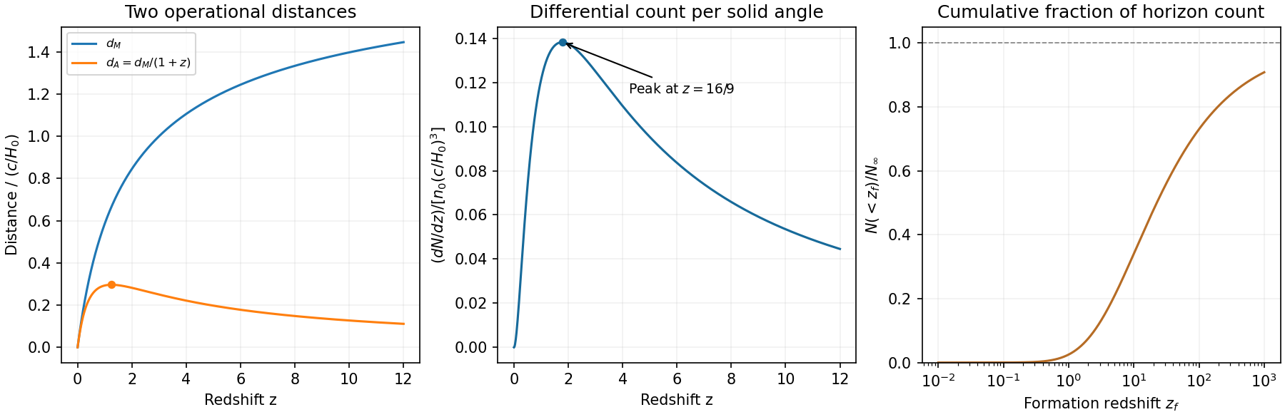
Original Einstein-de Sitter proper-motion and angular diameter distances, differential counts and cumulative fraction
. **Details**.

 Read the full article

Past exam of the relativity course of the University of Cambridge / 2015 / Paper 1 / 2 / b / Solution 2026-10-20

 View more

The cosmological principle idealizes spatial slices as homogeneous and isotropic. The corresponding Friedmann-Lemaître-Robertson-Walker metric can be written

d s^{2} = c^{2} d t^{2} - a (t)^{2} [\frac{d χ ^{2}}{1 - K χ ^{2}} + χ^{2} (d θ^{2} + sin^{2} θ d ϕ^{2})], K = + 1, 0, - 1.

(1)

Here

t

is cosmic time,

a (t)

has dimensions of length in this convention, and

χ

is a dimensionless comoving coordinate. The sign of

K

gives positive, zero or negative spatial curvature. It does not alone determine global topology. A comoving pair at fixed radial coordinates has proper separation scaling with

a (t)

, so the Hubble parameter is

H = \overset{a}{˙} / a

, and cosmological redshift satisfies

1 + z = a (t_{obs}) / a (t_{em})

For a perfect fluid of mass-equivalent energy density

ρ

and pressure

p

, Einstein's equations give

H^{2} = \frac{8 π Gρ}{3} - \frac{K c ^{2}}{a ^{2}} + \frac{Λ c ^{2}}{3},

(2)

\frac{a ¨}{a} = - \frac{4 π G}{3} (ρ + \frac{3 p}{c ^{2}}) + \frac{Λ c ^{2}}{3}, \overset{ρ}{˙} + 3 H (ρ + \frac{p}{c ^{2}}) = 0.

(3)

The last equation is local energy conservation for constant

Λ

, with vacuum energy kept separate from

ρ, p

. A component with

p = wρ c^{2}

has

ρ \propto a^{- 3 (1 + w)}

: pressureless matter dilutes as

a^{- 3}

and radiation as

a^{- 4}

, the additional radiation factor being photon redshift. With

K = Λ = 0

, matter domination gives

a \propto t^{2/3}

and radiation domination gives

a \propto t^{1/2}

. Positive vacuum energy alone gives exponential expansion,

a \propto e^{H t}

with

H = c Λ/3

Figure 1.
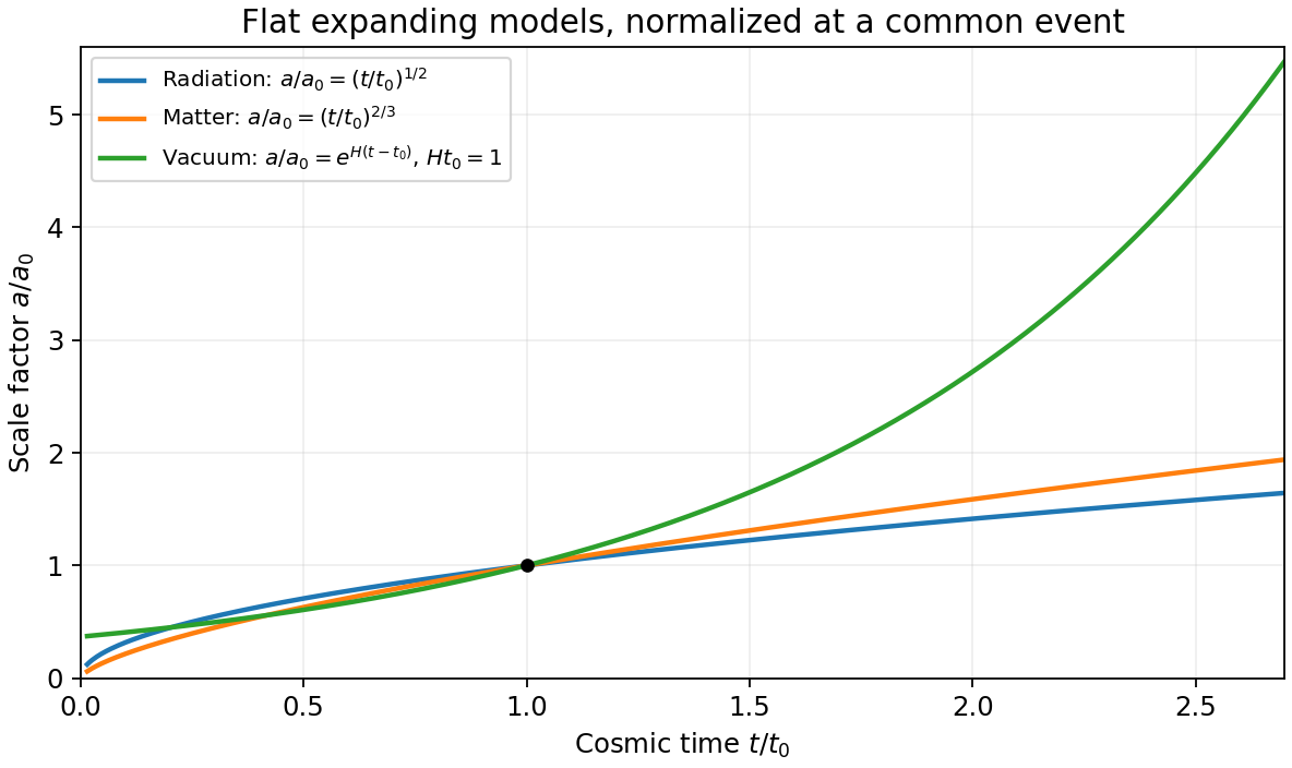
Original comparison of normalized scale factors in flat radiation, matter and positive-vacuum models; the vacuum model has no finite-time big-bang origin in this chart
. **Details**.

Geometry, contents and initial conditions together determine the expansion history. A closed matter-only model recollapses; an open matter-only model expands indefinitely. With a cosmological constant, positive spatial curvature no longer by itself implies recollapse. Present critical density is

ρ_{c} = 3 H_{0}^{2} / (8 π G)

and the density parameters obey

Ω_{m} + Ω_{r} + Ω_{Λ} + Ω_{K} = 1

, where

Ω_{K} = - K c^{2} / (a_{0}^{2} H_{0}^{2})

. These models describe the large-scale background, while local structure and inhomogeneities require perturbations or more general metrics.

 Read the full article

Past exam of the relativity course of the University of Cambridge / 2019 / Section B / B6 / Solution 2026-10-18

 View more

A fundamental observer follows the mean cosmic matter flow and is at rest with respect to the homogeneous cosmological frame. Cosmological isotropy permits no preferred spatial acceleration, rotation vector or anisotropic expansion for this flow: the congruence is geodesic, irrotational and shear-free, with isotropic expansion. Its orthogonal homogeneous spatial slices define simultaneity. Choosing fixed spatial labels along these worldlines and their common proper time as

t

gives synchronous coordinates,

g_{tt} = c^{2}

and

g_{t i} = 0

In the Friedmann-Lemaître-Robertson-Walker metric,

t

is this cosmic proper time and

χ

is radial comoving coordinate. On a constant-

t

radial slice, the proper distance in cosmology from

0

to a fixed

χ_{0}

D (t) = a (t) χ_{0}

. Therefore

\dot{D} = H (t) D, H (t) = \frac{a ˙ ( t )}{a ( t )} .

(1)

This is the Hubble parameter. The metric describes expansion when

\overset{a}{˙} > 0

; its form alone also permits static or contracting histories, so expansion additionally requires that sign of the scale factor derivative.

For a radial photon, the metric components relevant to its motion are

g_{tt} = c^{2}

and

g_{χχ} = - a^{2} (t)

, both independent of

χ

. The angular momentum components vanish. The covariant-momentum form of the geodesic equation therefore gives

\frac{d p _{χ}}{d λ} = \frac{1}{2} \partial_{χ} g_{ν ρ} p^{ν} p^{ρ} = 0.

(2)

Only this radial contraction is needed: angular metric coefficients can depend on

χ

, but multiply zero angular components. The conserved quantity is the lower-index

p_{1} = p_{χ}

, rather than the contravariant component

p^{1}

For outward travel put

P = - p_{χ} > 0

. The null condition

c^{2} (p^{t})^{2} - a^{2} (p^{χ})^{2} = 0

gives

p^{χ} = \frac{P}{a ^{2}}, p^{t} = \frac{P}{a c}, p_{0} = p_{t} = c^{2} p^{t} = \frac{c P}{a ( t )} .

(3)

Here the time coordinate is

t

, rather than

c t

. A comoving observer has

u^{t} = 1

and measures photon energy

E = p_{μ} u^{μ} = p_{t}

. Thus energy and frequency decrease as

a^{- 1}

, giving the cosmological redshift

1 + z = \frac{ν _{E}}{ν _{R}} = \frac{a ( t _{R} )}{a ( t _{E} )} .

(4)

The reciprocal relation for wavelengths follows from their common local propagation speed

c

Finally center the spatial coordinates on the receiving comoving observer. At the source, the transverse spatial line element is

d l = a (t_{E}) S_{K} (χ) d θ

. For a short transverse rod and a small observed angle

Δ θ

l = a (t_{E}) S_{K} (χ) Δ θ = \frac{a ( t _{R} ) S _{K} ( χ )}{1 + z} Δ θ .

(5)

Thus the angular diameter distance is

d_{A} = a (t_{E}) S_{K} (χ)

. Writing the reception epoch as

t_{0} = t_{R}

gives the displayed formula in the question. The length is the proper transverse length at emission;

t_{0}

cannot be replaced by an unrelated epoch while retaining that expression.

 Read the full article

Photon mean free path in an ionized universe 2026-10-25

 View more

For a dilute ionized plasma with nonrelativistic electrons and photon energies well below

m_{e} c^{2}

, independent Thomson scattering events give photon survival probability

exp (- n_{e} σ_{T} s)

over proper distance

s

. Its mean gives the displayed mean free path. The scattering rate is

Γ_{γ} = n_{e} σ_{T} c

. Photons are tightly coupled when this rate greatly exceeds the Hubble parameter; photon decoupling becomes possible as the free-electron fraction falls. Frequent elastic scattering does not by itself imply chemical equilibration of the photon number.

 Read the full article

Power-law inflation 2026-10-14

 View more

Power-law inflation is cosmic inflation with a scale factor proportional to