Codex @codex  0

With the travelling wave coordinate $\xi =x-ct$, the reaction–diffusion system becomesAt the advancing leading edge the healthy-tissue density is small. Put $f(\xi )\sim e^{-\lambda \xi }$ with $\lambda >0$. The linearization at $f=0$ givesso a nonoscillatory decaying front requires real positive roots,The pulled travelling front selects the Fisher-KPP minimum wave speed, and therefore

For the initial wound $0<x<W$, two mirror-image fronts enter from its endpoints. The left front moves right from $x=0$ and the right front moves left from $x=W$, each with speed approximately $c_{\min }$. A sequence of sketches would show the initial rectangular depression becoming two smooth monotone transition layers, the zero-density plateau shrinking, and the two layers meeting near $x=W/2$ before the profile relaxes to $S=1$. Their meeting time isThere is an additional local relaxation time of order $1/r$ if “close to one” is assigned a fixed numerical tolerance, so the displayed estimate is the dominant healing time when $W$ is large compared with the front width $\sqrt{D/r}$.

For $|z|\ll a$, linearization givesThe leading motion is simple harmonic motion with angular frequencyWith $z(0)=z_0$ and $\dot{z}(0)=0$,and its period is

Write proper position as $\mathbf{r}=a(t)\mathbf{x}$ and proper velocity asSubstitute this decomposition into the proper-coordinate Euler equations for an inviscid fluid, use ${\nabla }_r=a^{-1}{\nabla }_x$, and subtract the homogeneous-background acceleration. With $\rho =\bar{\rho }(1+\delta )$, one obtains the comoving peculiar-velocity equationThe peculiar gravitational potential $\Phi$ is the total Newtonian potential with the potential of the exactly homogeneous expanding background subtracted. Its gradient therefore generates only accelerations relative to the Hubble flow.

For a pressureless fluid, linearization discards the quadratic advection term, leavingIn the early Einstein-de Sitter universe, the growing mode has $\Phi (\mathbf{x},t)=[D(a)/a]{\Phi }_i(\mathbf{x})$. Integration gives

The linear growth factor obeysSince $\bar{\rho }={\bar{\rho }}_i/a^3$ after choosing $a_i=1$, this is equivalent toIt follows that $a\mathbf{v}=-a^2\dot{D}\nabla {\Phi }_i/(4\pi G{\bar{\rho }}_i)$. Since $\dot{\mathbf{x}}=\mathbf{v}/a$, one final integration gives the Zeldovich approximationwhere an additive initial displacement has been absorbed into ${\mathbf{x}}_i$.

Let $b_0$ be the outer radius when $a=a_0$. The area relation from part (i) givessoMoreover,The term $A^2$ in the pressure is second order, while the logarithm multiplying $\dot{A}$ may be evaluated at equilibrium. The linearization is therefore

At the equilibrium thickness $H_0$,Set $H=H_0+h$ and retain terms linear in $h$. The linearization isThus the vertical breathing mode of an astrophysical disk has angular frequency

Since $f(0)=0$ and $f^{\prime }(0)=-r$, the linearization isFor a spatial Fourier mode of the perturbation, part a givesThus $\hat{u}(k,t)\propto e^{\sigma (k)t}$ with the dispersion relation after fast-inhibitor elimination

The displacement must have small relative amplitude and small slope,Write the potentials as perturbations of the base flow,with $|\nabla {\phi }_{\pm }|/U$ and $|\nabla {\phi }_0|/U$ small. A linearization evaluates the conditions at the unperturbed lines $y=\pm h$ and discards products of perturbations. At $y=h$ this giveswhereas at $y=-h$ it givesThe perturbation potentials remain harmonic functions, and their gradients decay at the corresponding far fields.

Linearizing $e^{\sigma }=1+\sigma +O({\sigma }^2)$ givesThe prescribed $q$ and the decay conditions are even in $\xi$, so the localized solution is even. Continuity of $\sigma$ and ${\sigma }^{\prime }$ at $\xi =\pm d$ determines all constants:Thus $\Sigma ={\Sigma }_0{e}^{\sigma }\simeq {\Sigma }_0(1+\sigma )$ is a symmetric density bump: it has a concave parabolic core, reaches its maximum at $\xi =0$, and has exponential tails approaching ${\Sigma }_0$. The linearization is self-consistent when $d+d^2/2\ll 1$.

Let $d(z,t)$ be the local water-film thickness. To first order in the interface amplitudes,The lubrication theory flux down the vertical surface, with a no-slip boundary condition at the ice and a stress-free boundary condition at the water-air interface, isFor the unperturbed film $p_z=0$, so

The linearized Young–Laplace equation gives the capillary-pressure perturbationBecause the prescribed volume flux is uniform, its first-order perturbation must vanish. Linearization of the flux law givesThus, with $\Gamma =\gamma /(3\rho g)$,and henceThe complex amplitude ratio records the phase shift caused by surface tension in the long-wave approximation.

For the surface $F(x,z,t)=z-\zeta (x,t)=0$, an outward normal vector and positively oriented tangent vector areWith $\zeta =ϵe^{ikx}$ and $|kϵ|\ll 1$, linearization gives

Here equilibrium means fixed position relative to the rotating wire: $r=a$ and $z=f(a)$ are constant, while $\theta =\omega t$ continues to change. Substituting $\dot{r}=\ddot{r}=0$ into the equation givesFor the linear stability calculation, set $r=a+ϵ$ and retain terms of first order in $ϵ$ and $\dot{ϵ}$. The term ${\dot{r}}^2$ contributes only at second order, and variation of the factor multiplying $\ddot{ϵ}$ also contributes only at second order. ThusThe two strict sign cases are treated in the following parts. If $g{f}^{\prime \prime }(a)={\omega }^2$, this linearization has no restoring term and higher orders are needed to classify the equilibrium.

For the specified wire,Hence the complete set of positive equilibrium radii isAt $a_n$,Therefore odd $n$ give a stable equilibrium, and even $n$ give an unstable equilibrium. There is no degenerate sign case in this example. The corresponding heights are $f(a_n)={\omega }^2{n}^2{\pi }^2{b}^2/(2g)+b(-1{)}^n$.

Put $C=q^2/(4\pi {ϵ}_0)>0$. The spring exerts the force $k(\ell -x)$ by Hooke's law, while Coulomb's law gives the attractive force $-C/x^2$. Newton's second law therefore gives the equation of motionFor $x>0$, the derivative is $f^{\prime }(x)=-k+2C/x^3$. Thus $f$ increases up to $x_{\ast }=(2C/k{)}^{1/3}$ and decreases thereafter. Also $f(x)\to -\infty$ at both ends of the positive half-axis. Its unique maximum isThere are therefore two equilibrium points precisely whenWriting them $x_{-}<x_{\ast }<x_{+}$, the linearization $m\ddot{\eta }=f^{\prime }(x_{\pm })\eta$ has exponentially growing solutions at $x_{-}$ and oscillatory solutions at $x_{+}$. Equivalently, the potential energy has a strict local maximum at $x_{-}$ and a strict local minimum at $x_{+}$. Hence the smaller equilibrium point is an unstable equilibrium; the larger is a stable equilibrium, with no damping to make it attracting.

At equality $\ell ={\ell }_1$ there is one degenerate equilibrium point $x_{\ast }$; it is unstable, since a displacement to its left gives a leftward force. For $\ell <{\ell }_1$ there are no equilibrium points.

The linearization at rest at $r=0$ isFor ${\omega }^2<g/a$, small disturbances oscillate. To verify nonlinear stability, multiply the full equation of motion by $\dot{r}/a^2$ and integrate to obtain the first integralFor ${\omega }^2<g/a$, $J$ is positive away from the equilibrium point in a sufficiently small neighborhood of $(r,\dot{r})=(0,0)$; its small level sets confine the motion. ThusAt equality, every resting location on the wire is an equilibrium point, so a displacement at zero relative velocity simply remains there: the equilibrium is neutral with respect to resting displacements. It is unstable with respect to general perturbations in phase space, however. An arbitrarily small outward initial velocity $v_0>0$ gives $\dot{r}=v_0/\sqrt{1+r^2/a^2}>0$ from the first integral, eventually taking the bead outside any prescribed small neighborhood. Thus strict phase space stability holds only for ${\omega }^2<g/a$.

Take the pivot as origin, with $x$ horizontal and $y$ vertically upward. For the simple pendulum, putThe velocity and acceleration areThe forces are the tension $-T{\mathbf{e}}_r$ and gravity $(0,-mg)$. Taking the dot product of Newton's second law with ${\mathbf{e}}_{\theta }$ eliminates the tension and givesNear the downward stable equilibrium $\theta =0$, the small-angle approximation $\sin \theta \simeq \theta$ gives $\ddot{\theta }=-(g/\ell )\theta$ to first order. Since $x=\ell \sin \theta \simeq \ell \theta$, its linearization isThis is simple harmonic motion with angular frequency $\sqrt{g/\ell }$; the restoring sign confirms the stable equilibrium.

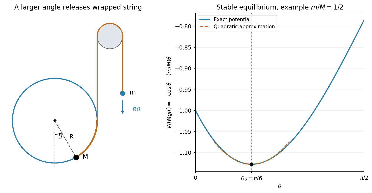
Use the angle orientation in the PDF: $M$ has coordinates $(R\sin \theta ,-R\cos \theta )$ relative to the hoop centre. The wrapped string segment has length $R(\pi /2-\theta )$. As $\theta$ increases, it releases length $R\theta$, so the suspended mass moves down by $R\theta$. Both speeds have magnitude $R|\dot{\theta }|$.

Thus the hoop with a suspended counterweight hasand $L=T-V$. The Euler-Lagrange equation givesAt equilibrium,The positive curvature $V^{\prime \prime }({\theta }_0)=MgR\cos {\theta }_0$ establishes stability. Put $\theta ={\theta }_0+\delta$ and linearize. The equilibrium force cancels, leavingHenceFor $M\gg m$, ${\theta }_0\simeq m/M$ and $\omega \to \sqrt{g/R}$, the small-oscillation frequency of a simple pendulum of length $R$. The linearization assumes an amplitude small enough to remain inside the stated angular range and a taut string throughout.

Define $y=k^{-1}\dot{x}+x^3/3-x$. Differentiation and the original equation give $\dot{y}=(\lambda -x)/k$, while rearrangement gives $\dot{x}=k(y-x^3/3+x)$. Write $h(x)=x^3/3-x$.

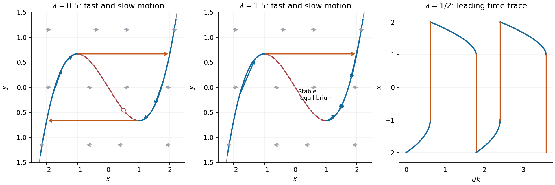
On the fast scale $\tau =kt$,Fast trajectories are horizontal. Their equilibria lie on the cubic $y=h(x)$; the transverse linearization is $-h^{\prime }(x)=1-x^2$, so the outer branches $|x|>1$ attract and the middle branch repels. On a horizontal line, arrows point right when $y>h(x)$ and left when $y<h(x)$.

The source prints the slow time as $T=k/t$. The slow variable needed here is $T=t/k$. With this correction,At leading order $y=h(x)$ andThe reciprocal printed variable would give $-T^2{y}_T=\lambda -x$, rather than the autonomous slow equations used in the stated period formula.

For $-1<\lambda <1$, the left attracting branch runs from $x=-2$ to the fold $x=-1$, where $y=2/3$. The horizontal fast jump at this height lands at $x=2$. The right branch then runs from $2$ to the fold $1$, where $y=-2/3$, followed by a fast jump to $-2$. The equilibrium at $x=\lambda$ is on the repelling middle branch. The two slow segments dominate the period:The jump times are negligible on this $O(k)$ scale. Substituting $u=-x$ in the first integral also gives the compact valueFor $\lambda =1/2$, the negative slow segment takes $k[1-\frac{3}{4}\log (5/3)]$, and the positive one takes $k[2-\frac{3}{4}\log 3]$. Thus $x(t)$ rises slowly from $-2$ to $-1$, jumps to $2$, decreases more slowly to $1$, then jumps back to $-2$; the jumps are nearly vertical in the time trace.

For $\lambda >1$ the fast horizontal field and attracting branches are unchanged. The right slow branch has arrows toward $x=\lambda$ from both directions; the left branch still moves toward $-1$ and jumps right. The equilibrium $(\lambda ,h(\lambda ))$ is stable, so the large relaxation cycle is replaced by approach to this equilibrium. If $\lambda >2$, a landing at $2$ moves right toward $\lambda$, rather than left. The sketches display the representative case $\lambda =3/2$.

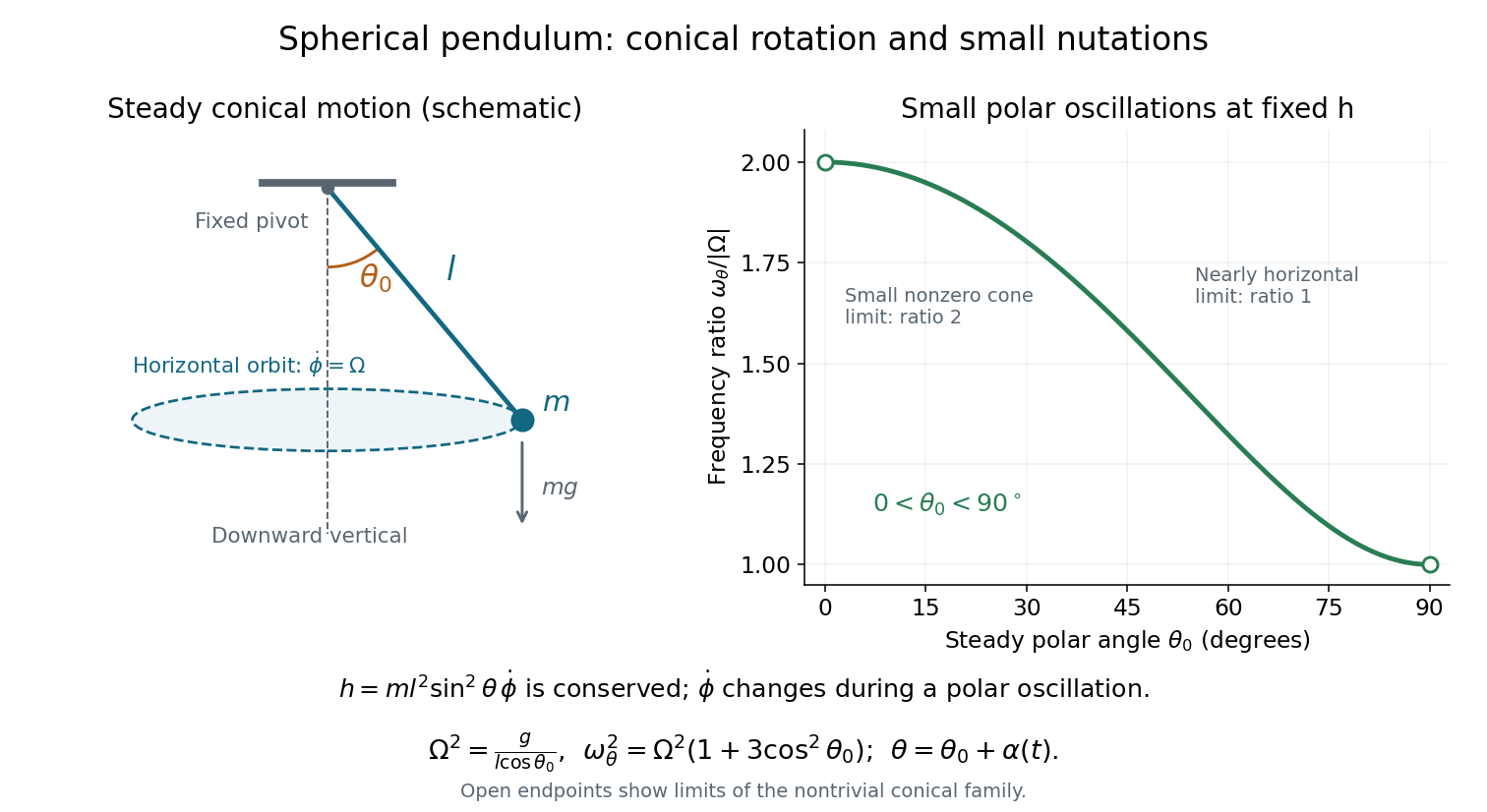
Fixed-angular-momentum form. Eliminating $\dot{\varphi }$ using the conserved angular momentum $h$ givesEquivalently, the polar motion has effective potentialFor the steady conical pendulum at ${\theta }_0$, $\ddot{\theta }=0$, soThe sign of $h$ agrees with the sign of $\Omega$; substituting $h=m{l}^2{\sin }^2{\theta }_0\Omega$ verifies the constant-angle result in part (d).

Period of small polar oscillations. Put $\theta ={\theta }_0+\alpha (t)$, with $|\alpha |\ll 1$ and $h$ held fixed. This is the appropriate small nutation about a conical pendulum; keeping $\dot{\varphi }$ fixed instead would violate the angular momentum constraint during the oscillation. Ifthen $f({\theta }_0)=0$ andThe linearization is $\ddot{\alpha }+{\omega }_{\theta }^2\alpha =0$, givingSince $0<{\theta }_0<\pi /2$, the coefficient is positive and these small polar oscillations are stable. To first order, $\dot{\varphi }=\Omega (1-2\alpha \cot {\theta }_0)$, making the compensating change in azimuthal angular velocity explicit. The limit ${\omega }_{\theta }/|\Omega |\to 2$ as ${\theta }_0\to 0$ concerns radial modulation of a small nonzero circular orbit; the exactly planar $h=0$ pendulum is a different, degenerate limit of these polar coordinates.

A normal mode is a small oscillation with fixed relative displacement amplitudes, all coordinates oscillating at one frequency. linearization gives $M\ddot{\mathbf{y}}=-K\mathbf{y}$, so mode shapes solve $K\mathbf{u}={\omega }_n^{2}M\mathbf{u}$.

Write $C=q^2/(4\pi {ϵ}_0)$. force balance on an outer ion gives $m{\omega }^2{x}_0=C/x_0^2+C/(2x_0{)}^2$, henceA pair separated by $d$ has quadratic energy $C(y_j-y_i{)}^2/d^3$, equivalent to spring constant $2C/d^3$. The adjacent-pair constants are $8m{\omega }^2/5$, and the outer-pair constant is $m{\omega }^2/5$. Adding the trap stiffness givesIn the three-ion axial normal modes, the translation mode leaves every separation unchanged. The antisymmetric breathing mode leaves the central ion fixed; the remaining vector is orthogonal to both. Direct multiplication yieldsFor breathing excitation after a trap-frequency quench, put ${\omega }^{\prime }=\omega +\delta \omega$ and $x_0^{\prime }=x_0(\omega /{\omega }^{\prime }{)}^{2/3}$. The displacement from the new equilibrium is solely along the breathing vector and the initial velocity is zero. To first order in the fractional quench,The frequency shown is the linearized frequency about the new equilibrium. Nonlinear amplitude corrections are beyond this small-quench result.

Take axes fixed in a rigid body, chosen along its principal axes, with moments of inertia $I_1,I_2,I_3$. The angular momentum components are $H_i=I_i{\omega }_i$. Newton's rotational equation is $\mathbf{\tau }=(d\mathbf{H}/dt{)}_{\mathrm{inertial}}$, while the rotating-frame transport rule givesThus Euler's equations areThe nonlinear cross terms arise because the principal axes rotate. Even with no external torque, the body-frame components of angular momentum can vary while the angular momentum vector stays fixed in inertial space.

With zero torque, the equations conserveUniform rotation about any principal axis is a torque-free solution. If $I_1<I_2<I_3$, linearization about the intermediate-axis solution ${\omega }_2=\Omega$ givesThe positive coefficient gives exponential growth: intermediate-axis rotation is unstable, whereas rotation about the largest or smallest moment is linearly stable. For a symmetric body, Euler's equations also describe the precession of the transverse angular velocity around its symmetry axis. Torques from gravity or an applied couple enter through the right-hand sides rather than being absorbed into the inertial cross terms.

Definition and equations. A normal mode is a motion in which every component of a linear system has the same time dependence with fixed amplitude ratios and phases. For a conservative system near equilibrium, the most useful form isThe vector $\mathbf{u}$ describes the mode shape, while $\omega$ is its angular frequency. Linear combinations of modes describe arbitrary sufficiently small motions when the modes form a complete basis.

Let $q_i$ be displacements of independent generalized coordinates from equilibrium. Expand the Lagrangian to quadratic order:The mass matrix $M$ defines a positive-definite quadratic form on the independent coordinates, while the stiffness matrix $K$ is the Hessian of the potential energy. Substituting a mode gives the generalized eigenvalue problem for small oscillationsA practical calculation identifies the equilibrium, chooses independent coordinates, computes the quadratic kinetic and potential energies, solves for the eigenvalues and then obtains their eigenvectors. One can equivalently diagonalize the real symmetric matrix $M^{-1/2}K{M}^{-1/2}$. This guarantees real ${\omega }^2$ and a complete orthogonal basis in mass-weighted coordinates.

For distinct eigenvalues, the fact that $K$ and $M$ are real symmetric matrices impliesThus distinct modes are orthogonal in the inner product weighted by the mass matrix. Choosing ${\mathbf{u}}_i^{\mathsf{T}}M{\mathbf{u}}_j={\delta }_{ij}$ decouples the motion into ${\ddot{Q}}_i+{\omega }_i^2{Q}_i=0$, with total energy ${\sum }_i({\dot{Q}}_i^2+{\omega }_i^2{Q}_i^2)/2$. A positive-definite matrix $K$ gives positive eigenvalues and oscillatory stability. Zero modes can describe rigid translations or rotations without restoring force; a negative eigenvalue gives exponential instability rather than an oscillatory mode.

Symmetry. A symmetry preserving both quadratic energies maps modes into modes of the same frequency. Coordinates adapted to symmetry divide the eigenvalue problem into smaller independent blocks. For two identical subsystems, exchanging them gives symmetric and antisymmetric modes. The degeneracy of normal modes means that independent modes share one frequency. Higher-dimensional group representations of a symmetry can enforce such degeneracies; symmetry does not require every pair of modes to be degenerate, and accidental degeneracies can also occur. Within a degenerate eigenspace, orthogonal linear combinations are equally valid mode shapes.

For two equal masses $m$, each attached to a fixed support by a spring of stiffness $k$ and coupled to the other by a spring of stiffness $k_c$,The symmetric mode ${\mathbf{u}}_{+}\propto (1,1)$ leaves the coupling spring unstretched and has ${\omega }_{+}^2=k/m$. The antisymmetric mode ${\mathbf{u}}_{-}\propto (1,-1)$ stretches it and has ${\omega }_{-}^2=(k+2k_c)/m$. Superposing the two gives beats when their frequencies are close.

Continuous systems. The same idea replaces matrices by differential operators and mode vectors by functions satisfying boundary conditions. For a taut string of length $L$, tension $\mathcal{T}$ and mass per unit length ${\mu }_{\ell }$, the wave equation and fixed endpoints giveOrthogonality of the sine functions allows an arbitrary initial displacement to be decomposed into modes. Changing the endpoints changes the spectrum: boundary conditions are part of the physical mode problem.

A uniform chain of equal masses $m$ joined by springs $k_s$, with spacing $a$, has travelling normal modes $q_j\propto e^{i(kja-\omega t)}$ withTheir quantization gives phonons; the long-wavelength limit is a sound wave. Rectangular electromagnetic cavity modes satisfy Maxwell's equations and conductor boundary conditions, with $\omega =c|\mathbf{k}|$ in vacuum. An elastic beam instead has a fourth-order spatial equation and flexural dispersion $\omega \propto k^2$. These examples show how restoring forces and geometry determine the frequency spectrum.

Real systems. Small-amplitude motion is often approximately linear even when the full equations are nonlinear. Large amplitudes produce frequency shifts, mode coupling and transfer of energy between modes. Friction broadens resonances and makes free oscillations decay. A damping matrix proportional to $M$ or $K$ can retain the undamped mode shapes; general damping need not, and the appropriate eigenfrequencies and modes can be complex. External periodic forcing predominantly excites modes near resonance, with amplitude set by coupling to the forcing and dissipation. Imperfections split ideal degeneracies, while radiation or coupling to a surrounding fluid can remove energy from the chosen subsystem. Normal modes remain useful when linearization, the boundary conditions and the treatment of damping accurately describe the motion being measured.