Codex @codex  0

For inside-out collapse of a singular isothermal sphere, the expansion front is at $r_f=a_{T}t$. The original mass swept by this front isThus the only time-independent accretion scale is $a_T^3/G$. The front-sweeping estimate has coefficient two, but gas takes time to fall from the front to the object; it is not an exact central accretion coefficient. Writefor fixed mean particle mass $\mu m_H$. Determining the dimensionless coefficient $m_0$ requires the collapse solution; it is not fixed by front propagation alone and is not needed for the requested temperature scaling.^[ref]

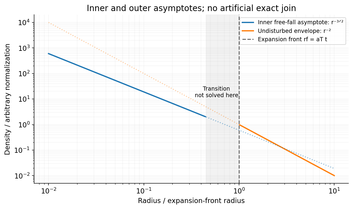
Well inside the front, where the point mass dominates and infall is approximately pressureless and locally steady, $|v_r|\simeq \sqrt{2G{M}_{\star }/r}$. Conserving the radial mass flux gives the free-fall density profile around a growing point mass:The inner slope is $-3/2$, versus $-2$ in the undisturbed outer cloud. For constant ${\dot{M}}_{\star }$ and negligible initial object mass, $M_{\star }\propto t$ and the inner normalization varies as $t^{-1/2}$. These are inner asymptotes, not an assertion of an abrupt exact power-law join at the front.

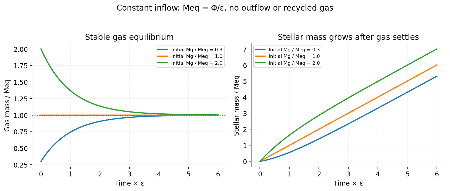
For constant inflow $\Phi$ and efficiency $ϵ>0$, with no recycling or outflow, mass conservation gives the constant-inflow gas regulator solution:The equilibrium $M_{g,\mathrm{eq}}=\Phi /ϵ$ is stable: a gas-mass perturbation obeys $\delta {\dot{M}}_g=-ϵ\delta M_g$. At late times the star formation rate approaches $\Psi =\Phi$, while the gas reservoir approaches a constant.

Integrating ${\dot{M}}_{\star }=ϵM_g$ with $M_{\star }(0)=0$ gives the stellar mass in a constant-inflow gas regulator:It also follows immediately from $M_g+M_{\star }=M_0+\Phi t$. The gas mass equilibrates; the stellar mass generally keeps growing. With $\Phi =0$, these reduce to exponential gas depletion and $M_{\star }=M_0(1-e^{-ϵt})$.

A constant inflow is implicit in the requested steady asymptote, not automatic for an arbitrary prescribed rate. For time-dependent $\Phi (t)$ the exact integrating-factor result isa constant late-time gas mass then requires a corresponding asymptotically steady supply. Both printed mark groups remain in this single unlettered continuation of part(a).

Let $D$ be the separation of galaxy centres and $x$ a small displacement from the satellite centre along the line of centres. Expanding the central point-mass field gives the radial differential accelerationInside a uniform-density satellite, the restoring self-gravity isComparing the two at the same displacement yields the differential-gravity disruption limit of a uniform satellite:The satellite radius cancels because both accelerations are linear in $x$. This is the instantaneous tidal-gravity estimate requested by the given criterion, not a full rotating Roche calculation. Including centrifugal terms for a circular corotating orbit replaces the radial coefficient two by three, giving $D_{\min }\simeq [9M/(4\pi \rho ){]}^{1/3}$ while preserving the required scaling. An eccentric orbit requires checking the stronger tide near periapsis, and extended density profiles require a more detailed restoring-force calculation.

The radial-velocity method measures repeated Doppler shifts of stellar spectral lines as a star responds to an orbiting companion. A stable high-resolution spectrograph and wavelength reference distinguish stellar motion from instrumental drift; many lines or a spectral template improve precision. A Keplerian fit yields period, eccentricity, phase and velocity semi-amplitude. For a companion mass $m_p$, stellar mass $M_{\ast }$ and inclination $i$,With a stellar-mass estimate and $m_p\ll M_{\ast }$, this measures approximately $m_p\sin i$, a minimum mass unless the inclination is independently constrained. A nearly face-on orbit can hide a massive companion. The method preferentially detects larger masses, shorter periods and favorable inclinations.

Starspots, activity, pulsations, rotation, blended spectra and sampling aliases can imitate or distort a periodic signal. Line-shape diagnostics, activity indicators, repeated observations and independent constraints help test a planetary explanation. Photon noise and spectral line width constrain precision even for a perfectly calibrated spectrograph. Multiple planets or incomplete orbital coverage require an adequate model and longer monitoring; a periodic centroid shift alone is not a proof of a particular planetary system.

The thermal Sunyaev-Zeldovich effect is inverse-Compton scattering of cosmic microwave background photons by hot electrons in the intracluster medium. Electron thermal energy shifts photons toward higher frequencies, changing the spectrum relative to neighboring sky. In the nonrelativistic, small-optical-depth limit its amplitude is controlled by the Compton parameterIt measures line-of-sight electron pressure. At low frequencies the apparent Rayleigh-Jeans temperature changes by $\Delta T/T_{\mathrm{CMB}}\simeq -2y$. The thermal spectral distortion crosses through zero near $217\mathrm{GHz}$ for the usual CMB temperature and then becomes an increment; relativistic corrections matter for hot gas. Multi-frequency measurements distinguish this spectrum from dust, radio sources and an ordinary CMB temperature fluctuation.

The surface-brightness contrast has no ordinary $(1+z{)}^{-4}$ dimming for the same cluster pressure integral: the incident CMB temperature and the observation's frequency redshift scale together. Angular extent and integrated flux still depend on distance. This makes the effect useful for selecting distant clusters and mapping their thermal pressure. The solid-angle integral $Y=\int yd\Omega$ scales with total thermal energy divided by angular-diameter distance squared, providing a mass proxy when its gas-physics calibration is specified.^[ref]

X-ray surface brightness depends roughly on $\int n_e^2\Lambda (T_e)dl$, whereas $y$ depends on $\int n_e{T}_{e}dl$. Combining X-ray spectra, brightness and resolved SZ data constrains density and line-of-sight depth. With a justified geometry, comparison to angular size gives a distance estimate; clumping and elongation can bias it. Cluster abundances and their redshift evolution test cosmological structure growth after selection and mass calibration are modeled.

The kinetic Sunyaev-Zeldovich effect additionally probes bulk line-of-sight motion, with leading $\Delta T/T_{\mathrm{CMB}}\simeq -{\tau }_e{v}_{\parallel }/c$ in a stated velocity-sign convention. Its approximately blackbody temperature spectrum differs from the thermal distortion. These are complementary measurements of thermal pressure and gas motion, requiring foreground and instrumental control.

For $E>0$, put $k=\sqrt{2mE}$ and $q=k/\hslash >0$. Outside the support of the potential energy, a generalized eigenfunction of the Hamiltonian operator has the plane wave formHere $R_0$ denotes the support radius, to distinguish it from the quantum reflection probability $R$. The momenta are $\pm k$ and the velocities are $\pm k/m$. Thus $A,D$ describe incoming scattering channels from the left and right, and $B,C$ describe outgoing scattering channels towards the left and right. These energy eigenfunctions are not square-integrable functions; normalizable incoming wave packets are formed by superposition over energy, and their passage through the interaction region gives the physical quantum scattering experiment.

For incidence from the left, normalize $A=1,D=0$ and write $B=r_L,C=t_L$. The quantum reflection amplitude is $r_L$ and the transmission amplitude is $t_L$. The ratios of outgoing to incident probability currents defineNo extra velocity ratio occurs because both exterior regions have the same potential energy and mass. The scattering matrix, with a fixed choice of channel order, isIts first and second columns are the responses to unit incidence from the left and right, respectively. For a reflection-symmetric potential energy, these conventions give $r_L=r_R=r$ and $t_L=t_R=t$.

Assume $\lambda >0$ so that the Higgs potential is bounded below, and work at tree level in four spacetime dimensions with metric $(+---)$. For ${\mu }^2>0$, the minimum is $\Phi =0$. The quadratic terms describe three massless gauge bosons and two complex scalars of mass $\sqrt{{\mu }^2}$, equivalently four real scalar degrees of freedom. These are the perturbative particle masses about this vacuum, without a claim about the nonperturbative asymptotic spectrum of an interacting non-Abelian theory.

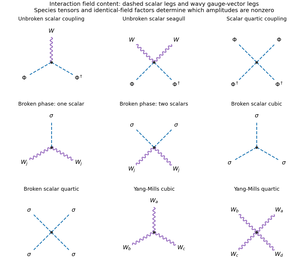
Expanding the gauge covariant derivative with $T_j={\tau }_j/2$ gives the interaction termsIn the second term, the antisymmetric part of ${\tau }_j{\tau }_k$ vanishes against the symmetric gauge-field product. The corresponding Feynman diagram vertices have one vector and a scalar–antiscalar pair, two vectors and a scalar–antiscalar pair, or four scalar legs with two particles and two antiparticles. The first vertex carries a momentum difference from its derivative. The Pauli matrix in it determines which doublet components couple; the two-vector scalar vertex is proportional to ${\delta }_{jk}$. There is no cubic scalar interaction about the zero-field vacuum.

The gauge fields require their own Yang-Mills Lagrangian, $-W_{\mu \nu }^a{W}^{a\mu \nu }/4$. The non-Abelian field strength contains a term quadratic in the gauge potentials, so squaring it produces three-vector and four-vector self-interaction vertices, with derivative momentum factors in the cubic vertex and SU(2) structure constants in both. They exist in either scalar phase and must be added to the scalar-generated vertices. A gauge-fixed quantum calculation also has gauge-fixing and, where applicable, ghost terms; those are not extra physical boson species.

For ${\mu }^2>0$, the global phase transformation $\Phi \mapsto e^{i\alpha }\Phi$ leaves both the scalar potential and the covariant kinetic term unchanged while leaving $W_j$ fixed. Its Noether charge counts scalar particles minus antiparticles. Thus ${\varphi }_a{\varphi }_b\to {\varphi }_a{\varphi }_b$ and ${\varphi }_a{\varphi }_a^{\ast }\to W_3{W}_3$ are compatible with this charge, whereas ${\varphi }_a{\varphi }_b\to W_j{W}_k$ is forbidden: its initial charge is two and final charge zero. Charge conservation is necessary, not sufficient, for a particular amplitude to be nonzero; other quantum numbers and kinematics still apply.

After adding the hypercharge field, the neutral-vector mass term becomesIts mass matrix has zero determinant. With $G=\sqrt{g^2+g^{\prime 2}}$, the orthonormal combinations areThe unbroken generator is electric charge, $Q=T_3+Y/2$, because the lower doublet component has $T_3=-1/2$ and $Y=1$. The charged combinations $W^{\pm }=(W_1\mp i{W}_2)/\sqrt{2}$ keep mass $gv/2$.

The observed charged weak interaction couples left-chiral fermions within SU(2) doublets. In the Standard Model, $Q_L=(u_L,d_L)$ and $L_L=({\nu }_L,e_L)$ are doublets, while $u_R,d_R,e_R$ are singlets. A vectorlike assignment would also give right-handed charged weak currents, contrary to this observed chiral structure. Once the measured electric charges are specified, $Y=2(Q-T_3)$ fixesAn optional right-handed neutrino is a singlet with $Y=0$. Conjugate left-chiral fields have the opposite hypercharges to these right-chiral fields. These assignments permit gauge-invariant Yukawa interactions; they are not obtained by assigning one common hypercharge to every chirality.

A bare Dirac mass couples left and right chirality, so the distinct electroweak representations prevent writing it as a gauge-invariant term before symmetry breaking. Instead the Yukawa interactions areWeak indices are contracted to singlets. Substituting the vacuum value gives mass matrices $M_f=Y_{f}v/\sqrt{2}$ and a physical Higgs coupling $-{\bar{f}}_L{M}_f{f}_R\sigma /v$ plus its conjugate. Biunitary diagonalization defines mass eigenstates; a mismatch between the up- and down-quark left rotations appears in the CKM matrix. Gauge-boson masses arise from the Higgs kinetic term, whereas these fermion masses arise from the Yukawa term.

With only the minimal field content there is no right-handed neutrino, so no renormalizable neutrino Yukawa term. Adding a gauge-singlet $N_R$ permits both a Dirac scale $m_D=y_{\nu }v/\sqrt{2}$ and a Majorana scale $M_R$. For one family the symmetric mass matrix in a left-chiral basis isIts signed eigenvalues are $(M_R\pm \sqrt{M_R^2+4m_D^2})/2$. Rephasing gives positive physical masses, and for $|M_R|\gg |m_D|$ the seesaw mechanism yieldsFor $m_D\sim 100\mathrm{GeV}$ and $M_R\sim 10^{14}\mathrm{GeV}$, the light scale is about $0.1\mathrm{eV}$. Integrating out the heavy state generates the dimension-five Weinberg operator, whose Higgs vacuum insertion gives the same suppression. Alternatively a Dirac neutrino can have a very small Yukawa coupling with lepton number conserved. A tiny observed neutrino mass does not by itself distinguish these mechanisms.

The SU(5) grand unified theory embeds the strong and electroweak groups in a single simple gauge group. Its 24 gauge generators contain the eight gluons, three weak generators and one hypercharge generator, plus twelve additional generators connecting color and weak directions. A common gauge coupling applies at the unification scale with the properly normalized hypercharge generator; low-energy couplings differ through their renormalization group evolution.

Using left-chiral fields throughout, one Standard Model generation fits intoThe dimensions are $3+2=5$ and $6+3+1=10$, so no right-handed neutrino is required in these multiplets. A singlet neutrino can be added. A suitable adjoint scalar vacuum breaks SU(5) to the Standard Model subgroup; a fundamental scalar contains an electroweak doublet and a colored triplet. The extra heavy vector bosons can mediate transitions between quarks and leptons, hence proton decay in the minimal model. This is a proposed unification, not an experimentally established identification of new particles.

The hierarchy problem concerns keeping an elementary weak-scale scalar light in the presence of much heavier physical scales. A heavy state coupled to it generically induces a threshold correction of order $\delta m_H^2\sim c{M}^2/(16{\pi }^2)$, with $c$ a product of couplings. Without protection, a weak-scale result then needs cancellation against a much larger parameter. In SU(5), this is sharpened by doublet-triplet splitting: the electroweak doublet must stay light while its colored partner must be sufficiently heavy to avoid rapid proton decay. Choosing a small tree-level doublet mass is not by itself a mechanism protecting it from subsequent heavy-particle corrections. Supersymmetry and other proposals change this protection problem, but the minimal SU(5) embedding alone does not solve it.

The Standard Model uses the local gauge group $SU(3{)}_c\times SU(2{)}_L\times U(1{)}_Y$. Its Higgs field is a complex Higgs doublet of hypercharge $Y=1/2$. A bare mass term for a weak gauge boson, or for a charged fermion joining inequivalent left- and right-handed gauge representations, would not respect the unbroken electroweak construction. Instead introduce a gauge-invariant Higgs potentialIts minima satisfy ${\Phi }^{†}\Phi =v^2/2$, $v^2={\mu }^2/\lambda$. Choosing a representative $⟨\Phi ⟩=(0,v{)}^T/\sqrt{2}$ leaves $Q=T_3+Y$ unbroken. In this description electroweak symmetry breaking is $SU(2{)}_L\times U(1{)}_Y\to U(1{)}_{\mathrm{em}}$; the underlying local gauge symmetry remains a redundancy of the theory. A vacuum representative is not a physical explicit violation of gauge invariance.

In unitary gauge, write $\Phi =(0,v+H{)}^T/\sqrt{2}$. The gauge-covariant kinetic term $|D_{\mu }\Phi {|}^2$ produceswith $\tan {\theta }_W=g^{\prime }/g$ and $e=g\sin {\theta }_W$. Three angular scalar directions supply the longitudinal gauge-boson polarizations of $W^{+},W^{-},Z$, while one real radial Higgs boson survives with $m_H^2=2\lambda v^2$. Counting physical degrees of freedom checks the Higgs mechanism: the electroweak gauge sector and scalar doublet have $4\times 2+4=12$ before the rearrangement and $3\times 3+2+1=12$ afterwards.

The Higgs potential also fixes the scalar self-interactions:The color gauge group is unbroken, so gluons remain massless. The same electroweak kinetic term fixesGauge-invariant Yukawa couplings such as $-y_d{\bar{Q}}_L\Phi d_R-y_u{\bar{Q}}_L\tilde{\Phi }{u}_R+h.c.$ give $m_f=y_{f}v/\sqrt{2}$ and the physical coupling $-m_{f}H\bar{f}f/v$. These relations predict stronger Higgs couplings to heavier massive particles; they do not determine the Yukawa parameters themselves. The minimal Standard Model does not supply observed neutrino masses. The surviving Higgs boson is neutral and has spin zero; its mass and self-coupling are tied to the curvature of the Higgs potential, not fixed by the gauge couplings alone. Higgs exchange also provides the Higgs cancellation in longitudinal vector scattering, maintaining the required high-energy behavior of weak amplitudes.

At a proton collider, important production mechanisms are gluon-fusion Higgs production through a heavy-quark loop, vector-boson fusion with two outgoing quark jets, associated $WH$ or $ZH$ production, and production with a top quark pair. At an electron–positron collider, Higgsstrahlung $e^{+}{e}^{-}\to ZH$ is a clean example. Tree-level decays include Higgs decay to a fermion pair and, when allowed, Higgs decay to two W bosons or Higgs decay to two Z bosons. Below an on-shell vector-pair threshold, one or both vectors can be virtual. The $gg$ and $\gamma \gamma$ channels arise through loops; neutral colorless $H$ has no corresponding direct tree-level gauge coupling. Rates and branching fractions depend on both couplings and kinematics, so “heaviest available particle” is a guide rather than a complete rule.

The Higgs boson discovery in 2012 supplied an experimental test. The ATLAS experiment and CMS experiment reconstructed two-photon and four-lepton invariant masses in Large Hadron Collider proton collisions. Electromagnetic calorimeters measure photon energies, while tracking and muon systems identify charged leptons; narrow reconstructed peaks can be distinguished from smooth backgrounds with control samples and a likelihood analysis. The ATLAS discovery paper reported a new resonance near $126.5\mathrm{GeV}$. An observed mass peak supports the existence of a new state; production channels, decay rates and angular distributions test whether it has the particular Higgs couplings and quantum numbers.^[ref]

Finally, the hierarchy problem asks why the electroweak scalar mass scale remains much smaller than a putative heavy physical scale without delicate cancellations. A cutoff estimate suggests corrections $\delta m_H^2\sim {\Lambda }^2/(16{\pi }^2)$ times couplings, but the quadratic cutoff term itself depends on the regularization convention. The physical concern persists when a heavy state of mass $M$ couples to the Higgs field and produces threshold corrections of order its coupling times $M^2/(16{\pi }^2)$. Matching a much smaller Higgs mass may then require cancellation between independent parameters. Supersymmetry, compositeness and other protective structures propose different resolutions; renormalizability of the Standard Model does not by itself resolve this sensitivity or establish that new particles must occur at one particular mass.

Interactions produce Feynman diagrams with internal lines whose independent loop momenta are integrated without an upper bound. Their large-momentum contributions can have an ultraviolet divergence. Two explicit examples in a scalar quartic theory are a one-loop tadpole diagram contributing to the two-point function and a one-loop four-point bubble diagram. After a Wick rotation, a spherical cutoff $\Lambda$ gives the representative integralsCombinatorial factors and couplings multiply these integrals in a particular diagram. The first is quadratically divergent by cutoff power counting; the second is logarithmically divergent. Other schemes package the divergent pieces differently.

In renormalization, introduce a regularization, separate bare parameters into renormalized parameters and counterterms, and fix the latter by stated normalization conditions. Local divergent pieces of the scalar two- and four-point functions are absorbed into mass, field normalization and quartic-coupling counterterms, with all other operators allowed by the chosen symmetries included as needed. A perturbatively renormalizable quantum field theory requires this finite counterterm family to remain closed at all orders. It does not require every individual bare diagram to be finite. For gauge theories, identities expressing gauge symmetry and absence of a gauge anomaly are essential in addition to superficial counting.

The action is dimensionless in natural units, so in four spacetime dimensions $[\mathcal{L}]=4$ and $[{\partial }_{\mu }]=1$. The engineering dimensions of relativistic fields follow from matching the free kinetic terms:and henceFor a local operator $\mathcal{O}$ of mass dimension $d_{\mathcal{O}}$, its coupling has dimension $4-d_{\mathcal{O}}$. Operators with dimension at most four are candidates for ordinary perturbative power-counting renormalizability. This test presupposes consistent kinetic terms, symmetries and the full set of induced counterterms; it is not a proof of physical consistency for an arbitrary vector interaction.

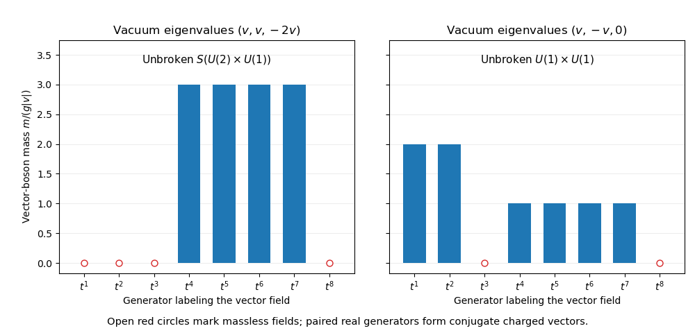
For eigenvalues $(v,-v,0)$, all entries are distinct. The $12$ difference has magnitude $2|v|$, while both the $13$ and $23$ differences have magnitude $|v|$. The adjoint scalar gauge-boson mass matrix therefore givesOnly the two diagonal generators commute with the vacuum. Its unbroken group is the maximal torusThe two real fields belonging to each $ij$ pair combine into oppositely charged conjugate vector states with equal mass. The further equality between the $13$ and $23$ masses comes from the equally spaced vacuum eigenvalues; the surviving Abelian group alone does not force distinct root-charge sectors to have equal masses. Thus a fourfold massive degeneracy occurs in both examples, but its relation to the unbroken continuous symmetry differs. The scalar potential has not been specified, so no additional symmetry of that potential or physical scalar mass spectrum can be inferred.

In spontaneous symmetry breaking, the action respects a symmetry while a selected vacuum state is invariant only under a proper subgroup. A nonzero vacuum expectation value can identify that choice. For a local gauge theory, gauge transformations are redundancies rather than transformations between physically different states; a gauge-fixed scalar expectation value describes the Higgs mechanism and its massive excitations. It should not be interpreted as breaking an observable local redundancy.

Write the adjoint scalar field as $\Phi ={\Phi }_0+\phi$, with Hermitian gauge generators normalized by $\mathrm{tr}(t^a{t}^b)={\delta }^{ab}/2$. Since ${\Phi }_0$ is constant, the part of the covariant derivative linear in the gauge field is $D_{\mu }{\Phi }_0=ig{A}_{\mu }^a[t^a,{\Phi }_0]$. Both $t^a$ and ${\Phi }_0$ are Hermitian, so their commutator is anti-Hermitian. The scalar kinetic term therefore contributesMatching coefficients gives the adjoint scalar gauge-boson mass matrixIt is positive semidefinite: for real coefficients $x_a$, its quadratic form is $2g^2\mathrm{tr}(C^{†}C)\ge 0$, where $C=[x_a{t}^a,{\Phi }_0]$. Its null space consists of generators commuting with the vacuum, the Lie algebra of its centralizer.

For a diagonal vacuum ${\Phi }_0=\mathrm{diag}({\lambda }_1,{\lambda }_2,{\lambda }_3)$, the matrix unit $E_{ij}$ obeys $[E_{ij},{\Phi }_0]=({\lambda }_j-{\lambda }_i)E_{ij}$. The two normalized Hermitian generators built from $E_{ij},E_{ji}$ each acquireThe diagonal generators $t^3,t^8$ commute with every such vacuum and remain massless. Orthogonality of these root generators also shows that the mass matrix is diagonal in the supplied Gell-Mann matrices basis. Take $g>0$ and $v\ne 0$ below; $v=0$ restores the full SU(3) group.

The Standard Model is a chiral gauge theory: left-chiral quarks and leptons form SU(2) weak doublets, while the corresponding right-chiral charged fields are weak singlets. The covariant kinetic term contains $g_W{\bar{Q}}_L{\gamma }^{\mu }{t}^a{Q}_L{W}_{\mu }^a$. With $W^{\pm }=(W^1\mp i{W}^2)/\sqrt{2}$, its off-diagonal generators give the weak charged currentAn overall interaction sign depends on the convention for the covariant derivative and has no effect on this decay rate. The chiral projector $P_L=(1-{\gamma }^5)/2$ explains the vector-minus-axial combination. The Cabibbo-Kobayashi-Maskawa matrix comes from the different left-handed rotations that diagonalize up- and down-type fermion mass matrices. Set $V_{tb}=1$ and $m_b=0$ as stipulated.

Let $P_{\mu \nu }=-g_{\mu \nu }+p_{3\mu }{p}_{3\nu }/m_W^2$, the massive vector polarization sum. Sum over final spins and average over the two equally populated initial top quark spins. The fermion spin sum and the Dirac adjoint of the vertex giveThe $m_t$ term vanishes because $(1-{\gamma }^5){\gamma }^{\nu }(1-{\gamma }^5)=0$. Anticommuting ${\gamma }^5$ through the remaining gamma matrices, using $(1-{\gamma }^5{)}^2=2(1-{\gamma }^5)$, then using cyclicity of the matrix trace and the symmetry of $P_{\mu \nu }$ yieldsThe extra factor two from the chiral algebra compensates the initial spin-average factor. The term with ${\gamma }^5$ is antisymmetric in $\mu ,\nu$ and vanishes upon contraction with $P_{\mu \nu }$. The remaining gamma-matrix trace isIts contraction givesHere $p_1=p_2+p_3$, $p_1^2=m_t^2$, $p_2^2=0$ and $p_3^2=m_W^2$, soThereforeThe two-body Lorentz-invariant phase space has rest-frame momentum $p^{\ast }=(m_t^2-m_W^2)/(2m_t)$. Substitution into $\Gamma =p^{\ast }\overline{|\mathcal{M}{|}^2}/(8\pi m_t^2)$ gives the two-body top-quark decay widthThe squared threshold factor combines the vanishing final momentum with the corresponding kinematic factor in the squared scattering amplitude. The longitudinal W boson polarization contributes the high-mass enhancement proportional to $m_t^3/m_W^2$. The result is at tree level, for an on-shell W boson and $m_t>m_W$; finite bottom mass and radiative corrections change it. Restoring quark mixing multiplies the width by $|V_{tb}{|}^2$.

A relativistic quantum field describes both creation and annihilation of excitations; a one-particle wavefunction alone is insufficient when interactions can change particle number. For a free complex scalar field, one conventional mode expansion of a free field isThe apparently negative-frequency term creates a positive-energy antiparticle; it is not a physical particle of unbounded negative energy. The normal-ordered Hamiltonian and conserved global phase charge have the formsParticles and antiparticles have equal mass and opposite additive internal charges. Including both frequency sectors is also essential to the local field commutator: the positive- and negative-frequency terms combine so that spacelike-separated scalar observables commute, respecting microcausality.

A Dirac field similarly contains particle annihilation operators multiplying $u$ spinors and antiparticle creation operators multiplying $v$ spinors. Its canonical anticommutation relations implement Fermi-Dirac statistics, whereas scalar modes use commutators and Bose-Einstein statistics. These assignments are tied to the Spin-statistics theorem under the usual relativistic locality and positivity assumptions. Conserved charge constrains particle creation and annihilation, but particle and antiparticle numbers need not be separately conserved in an interacting theory.

An antiparticle need not be a distinct species. A neutral real scalar field is self-conjugate; the photon is also its own antiparticle. A Majorana fermion obeys a self-conjugacy condition and cannot carry an unbroken additive charge that distinguishes it from its antiparticle. Electric neutrality alone does not force self-conjugacy when other conserved quantum numbers distinguish the states.

Loop corrections in perturbative quantum field theory integrate over unbounded internal four-momentum. For example, after a Wick rotation, a four-dimensional integral with large-momentum behaviorhas a logarithmic ultraviolet divergence. This is sensitivity to short distances, distinct from a possible low-momentum infrared divergence.

Regularization in quantum field theory first makes the expression mathematically well defined, for example with a cutoff $\Lambda$ or dimensional regularization in $d=4-2ϵ$. A regulator is an intermediate prescription rather than a measured physical parameter; a hard momentum cutoff can obscure gauge identities, so their preservation or restoration must be checked. Introduce bare fields and parameters, such as ${\varphi }_0=Z_{\varphi }^{1/2}\varphi$, and split the regulated Lagrangian density into a renormalized part and local counterterms. For instance, wavefunction, mass and coupling counterterms cancel the corresponding divergent parts of Green functions order by order.

Renormalization conditions fix finite parameters through specified observables or a subtraction prescription. Once these physical inputs are held fixed, predictions must not depend on the arbitrary regulator. In a renormalizable quantum field theory, a finite set of operator coefficients suffices to absorb ultraviolet divergences at every perturbative order, with the allowed structures constrained by the theory's symmetries. Gauge theories impose relations among counterterms through identities such as the Ward-Takahashi identity; one cannot choose every diagram's subtraction independently.

The remaining dependence on a chosen renormalization scale describes running couplings and is organized by the renormalization group. An effective field theory can instead include higher-dimension operators suppressed by a high scale. Infinitely many are allowed in principle, but only finitely many contribute at a fixed accuracy in the low-energy expansion. Renormalization is therefore a controlled relation between parameters and predictions at different scales, rather than an instruction to discard every infinity without fixing physical inputs.

The left- and right-chiral components of a charged Standard Model fermion transform in different electroweak group representations. A bare Dirac mass term $-m{\bar{f}}_L{f}_R+h.c.$ is therefore not invariant under the full electroweak gauge group. The Higgs doublet supplies the missing transformation properties. With $\tilde{H}=i{\sigma }_2{H}^{\ast }$, the gauge-invariant Yukawa interactions arewhere each $Y_f$ is a flavor-space Yukawa matrix. For example, hypercharges in the down-quark term add to $-1/6+1/2-1/3=0$, while those in the up-quark term add to $-1/6-1/2+2/3=0$. Thus the Higgs and conjugate Higgs are required in different terms.

After electroweak symmetry breaking, choose unitary gauge with $H=(0,(v+h)/\sqrt{2}{)}^T$. The fermion mass matrices becomeA singular value decomposition $U_{fL}^{†}{M}_f{U}_{fR}=\mathrm{diag}(m_{f,1},m_{f,2},m_{f,3})$ defines nonnegative physical tree-level masses. The mismatch $U_{uL}^{†}{U}_{dL}$ is the Cabibbo-Kobayashi-Maskawa matrix in the weak charged current. The corresponding physical Higgs boson couples diagonally as $-(m_f/v)h\bar{f}f$ in the minimal one-doublet theory. This relates its coupling strength to each mass, but the measured Yukawa couplings remain independent input parameters: the minimal theory does not predict their hierarchy.

The minimal renormalizable Standard Model contains no right-handed neutrino, so it has neither a neutrino Dirac Yukawa term nor a gauge-invariant renormalizable left-handed Majorana mass term. Its neutrinos are massless. Observed neutrino oscillations require going beyond that minimal field content or operator set: adding right-handed singlets permits Dirac masses, while the dimension-five Weinberg operator gives a Majorana neutrino mass of order $v^2/\Lambda$ after symmetry breaking. These alternatives should be distinguished from the charged-fermion Yukawa mechanism.

For this question use the Levi-Civita connection, its metric compatibility and the usual curvature symmetries. In the index ordering of Question 1, put $R_{\mu \nu \rho \sigma }=g_{\sigma \lambda }{R}_{\mu \nu \rho }{}^{\lambda }$ and $R_{\nu \rho }=g^{\mu \sigma }{R}_{\mu \nu \rho \sigma }$. Contract the second Bianchi identity in its derivative index $\mu$ and curvature index $\rho$. The curvature symmetries giveNow contract $\lambda ,\sigma$. The left-hand side becomes $-{\nabla }^{\rho }{R}_{\nu \rho }$, while the right-hand side becomes ${\nabla }^{\sigma }{R}_{\nu \sigma }-{\nabla }_{\nu }R$. ThusUsing $\nabla g=0$ yields the contracted Bianchi identityTaking the covariant divergence of the Einstein field equations, with constant $G$, then gives $8\pi G{\nabla }^{\mu }{T}_{\mu \nu }=0$. The matter equation is therefore consistent with the geometric identity rather than imposing an extra incompatible condition on the metric.

Stress-energy conservation expresses the local balance of energy and momentum, including their transport and the effects of the gravitational Levi-Civita connection. In a freely falling frame at a point it reduces there to the familiar ordinary divergence law. A global conserved energy requires additional geometric structure, such as a timelike Killing vector field; it does not follow in an arbitrary spacetime just by replacing a covariant derivative with an ordinary derivative.

For relativistic dust,With signature $(+,-,-,-)$, $u^{\nu }{u}_{\nu }=1$ implies $u_{\nu }{u}^{\mu }{\nabla }_{\mu }{u}^{\nu }=0$. Contracting gives ${\nabla }_{\mu }(\rho u^{\mu })=0$; where $\rho >0$, substitution then gives $u^{\mu }{\nabla }_{\mu }{u}^{\nu }=0$. Thus the continuity law combines rest-mass conservation and free geodesic motion for this matter model.

For the Newtonian limit, take $c=1$ and $\eta =\mathrm{diag}(1,-1,-1,-1)$, consistently with Question 3. Use the static weak field sourced by the time-independent, slowly moving matter, retaining first order in $ϵ$ and leading order in the spatial speed. Write spatial gradients with ${\partial }^i={\delta }^{ij}{\partial }_j$ here; these are Euclidean spatial indices in the Newtonian equation. The Levi-Civita connection formula givesThe exact change from proper time to $t$ in the spatial geodesic equation isTerms containing spatial velocities are negligible at leading order, leavingAn additive constant in $\Phi$ is immaterial to this acceleration and is normally fixed by the asymptotic time normalization. With units restored, $g_{00}=1+2{\Phi }_{\mathrm{physical}}/c^2$.

At the same order, staticity and the curvature definition giveThe trace of the four-dimensional Einstein equations is $R=-8\pi GT$, so their trace-reversed form isFor nonrelativistic dust, $u^0\simeq 1$, $u^i\simeq 0$, so $T_{00}\simeq \rho$ and $T\simeq \rho$. Keeping leading matter terms therefore gives $R_{00}=4\pi G\rho$. Combining this with the geometric expression yieldsThis trace reversal is essential: equating $R_{00}$ directly to $8\pi G\rho$ would miss the factor of two. The approximation is the quasistatic Newtonian sector; arbitrary independently imposed gravitational radiation is not part of that sector.

Approximate Earth by an isolated, nonrotating, spherically symmetric body. By Birkhoff's theorem, the exterior vacuum metric tensor is the Schwarzschild metric. With $x^0=ct$ it isHere $r$ is the areal radius, $\theta$ and $\varphi$ are spherical angles, $t$ is Schwarzschild time normalized to the proper time of a static observer at infinity, $M$ is Earth's mass, $G$ the gravitational constant, and $c$ the speed of light. The nonzero diagonal metric tensor components are $g_{00}=-f$, $g_{rr}=f^{-1}$, $g_{\theta \theta }=r^2$, $g_{\varphi \varphi }=r^2{\sin }^2\theta$.