Put . The hyperbolic tangent identity gives . Taking a compatible branch of the complex logarithm givesAs an identity for a single-valued inverse hyperbolic tangent, this requires consistent branch cuts; one cannot choose unrelated logarithm branches on the two sides. Near the branch with value zero is fixed by . The full inverse relation also allows , , and are singular points.
Expand the sine of the complex number using hyperbolic functions:Its squared complex modulus isTaking nonnegative square roots proves . Equality holds exactly when .
Use the Levi-Civita symbol and Einstein summation convention. The tensor contraction , expressed through the Kronecker delta, givesThe last two contractions are dot products, proving the vector triple product identity .
Choose the linear relationThen the displayed tensor contraction is , precisely the th vector component of by the vector triple product identity. The matrix need not be a symmetric matrix.
The characteristic equation of the damped harmonic oscillator is . In the underdamped case its roots are , where . Thus the exact real solution is . For , , giving the requested leading approximationFor mass and spring constant , the mechanical energy is . Differentiating and using the differential equation gives . In particular, energy decay of a viscously damped harmonic oscillator is not an exact pointwise exponential decay: at a turning point. To leading order in , the period average isThe quality factor is . Using the period and the small fractional loss gives . Equivalently, the energy-decay definition yields the same leading result. Replacing by in the oscillatory phase is not uniform over arbitrarily long times; its phase error is .
For and a nonzero solution, set . Since , multiplying the Bernoulli differential equation by gives the linear ordinary differential equationAn integrating factor gives . Recover from on an appropriate real or complex branch. This substitution can omit the zero solution, which must be checked in the original equation. For , no substitution is needed: is already a linear ordinary differential equation.
Work on an interval with . When , let . The resulting linear ordinary differential equation and its integrating factor areIntegration gives . The real nonzero solutions and the separately checked zero solution are thereforeFor , separation in the linear ordinary differential equation gives , henceHere already includes the zero solution. Division by is why these formulas are stated on intervals excluding zero; the original equation requires if a classical solution is to extend through zero.
Write the matrix trace in Einstein summation convention:The entries are scalars, so their multiplication commutes, and the two summed indices may be relabelled. The argument works for square matrices of any finite size, and also for rectangular of compatible opposite shapes.
Let with . A vanishing commutator gives , so belongs to the eigenspace . This is eigenspace invariance for commuting linear maps. A nondegenerate eigenvalue has a one-dimensional eigenspace, so for a scalar ; is allowed. Therefore is also an eigenvector of . Without the simple-eigenvalue condition, can mix vectors inside a larger eigenspace, and an arbitrarily chosen eigenvector of need not be an eigenvector of .
For Hermitian matrices, and , soThe commutator is an anti-Hermitian matrix. Consequentlymakes . More generally, any nonzero purely imaginary works. For a nonzero commutator this is also necessary if is to be Hermitian: comparing the Hermitian adjoint equations gives .
The characteristic polynomial factors as . Thus in algebraic multiplicity. An orthonormal basis of corresponding eigenvectors isDirect multiplication verifies , , . Their mutual Hermitian inner products vanish and each has norm one, which proves linear independence. For the repeated eigenvalue, Gaussian elimination givesHence . The second equality follows from the rank-nullity theorem and agrees with the two-dimensional eigenspace. A repeated eigenvalue alone would not imply a two-dimensional eigenspace for an arbitrary matrix; here the Hermitian matrix is diagonalizable.
For a purely imaginary candidate , , the imaginary part of the polynomial is . The candidate is not a root, while both make the real part zero. The resulting factorization into quadratic polynomials givesThe roots of a polynomial sum to and have product , as required by Vieta's formulas for a monic quartic with cubic coefficient and constant coefficient .
Expand using De Moivre's theorem, then divide its imaginary and real parts by . With , this givesThe quotient holds where its denominator and are nonzero. At , use the undivided real-part identity: implies . Thus . Since , the smaller positive value applies:This limiting step avoids treating an undefined value of as an ordinary finite number.
A plane through with nonzero normal vector consists of the position vectors satisfying . Thus , with . When is a unit vector, is the signed distance from the origin in the direction ; for an unnormalized normal vector, that distance is . The displacement within the plane is perpendicular to .
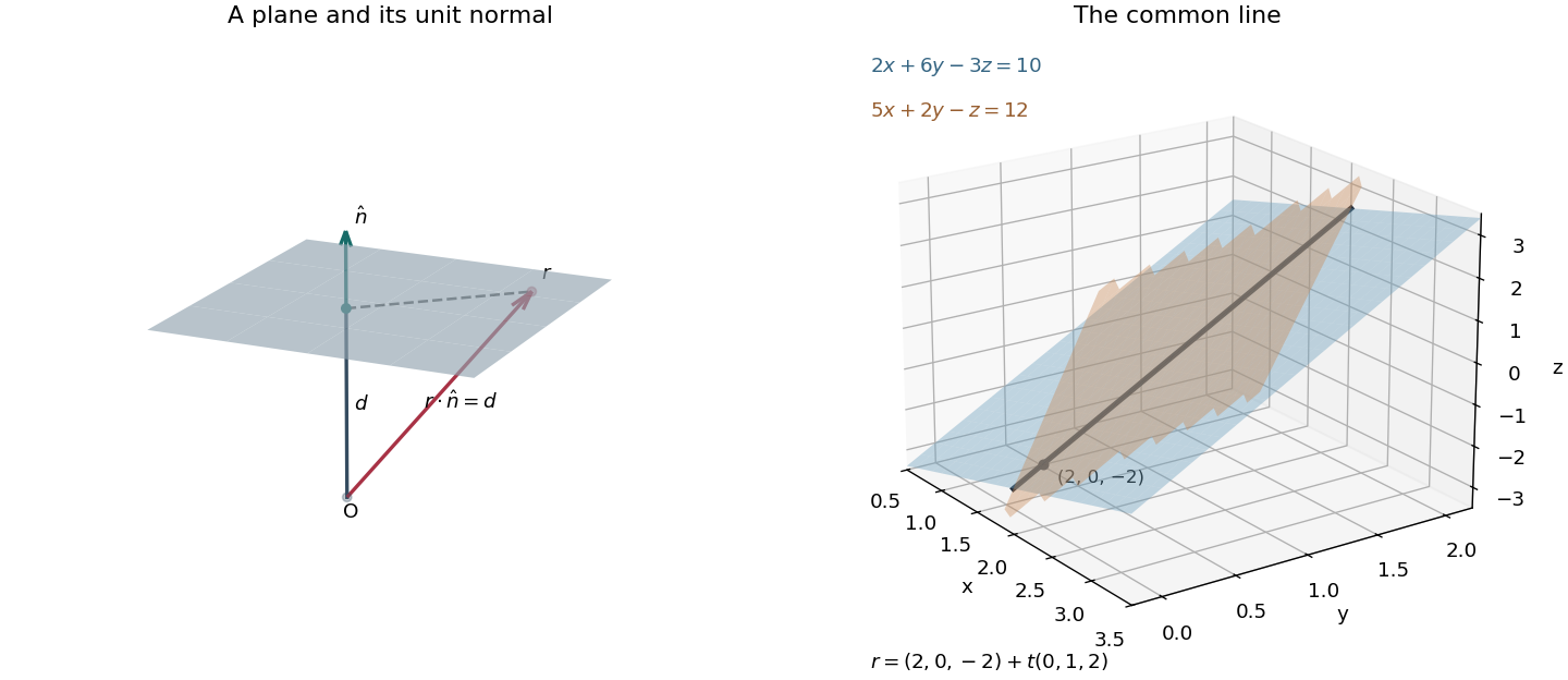
A unit normal vector and signed plane distance, followed by the intersection of two planes as a straight line
. Details. The cross product of the two normal vectors is , so their intersection of two planes has direction . Eliminating gives , and substitution then gives . Thus the Cartesian constraints and parametric equation of a straight line areThere is no valid division by a zero component in a symmetric ratio form; retaining explicitly handles that component.
The characteristic equation gives the complementary function . Write the forcing as . The method of undetermined coefficients gives for the first term. Because already belongs to the homogeneous solution, resonance in a differential equation requires a trial for the second; substitution gives . Therefore
Substitute the power series and its termwise derivatives into the ordinary differential equation. The coefficient of , for , isThe bracket factors as , so the power-series solution of a differential equation satisfiesThe odd and even recurrence relations terminate: , , and , , . Thus the full solution is . The two polynomials have independent initial data at zero, and the leading coefficient never vanishes on the real axis, so every real solution of a differential equation for this equation is their linear combination on the entire real axis. The given initial data select , :
The th column of the matrix representation of a linear map is the coordinate vector of the image of the th basis vector:Define by , so its columns express the new basis vectors in the old basis. For every vector, . Applying in either coordinate system gives , proving the change of basis formulaTo make diagonal, choose the columns of to be linearly independent eigenvectors of , expressed in the basis, and put their corresponding eigenvalues on the diagonal in the same order. This is possible precisely when is a diagonalizable matrix over the stated field; an eigenbasis need not exist over an arbitrary field.
The linear system of differential equations has matrixThe columns of are eigenvectors of . The change of basis therefore gives , , with independent first-order linear differential equationsThe initial velocity gives , . Transforming back, , yields the real velocity vector componentsThese also cover . Complex coordinates have decoupled a real rotation without making the physical velocity complex.
Adopt the convention that an inner product is linear in its second slot. Over , it is a symmetric bilinear form with , equality only for . Over , a Hermitian inner product obeysThese imply conjugate linearity in the first slot: . The strict positivity condition distinguishes an inner product from a general Hermitian form.
Expand the vector in the orthonormal basis, . Using linearity in the second slot and the Kronecker delta givesExpanding both vectors and using conjugate linearity in the first slot therefore givesAn orthonormal set that is not a basis would recover only the coordinates of the orthogonal projection onto its linear span; here the vectors span .
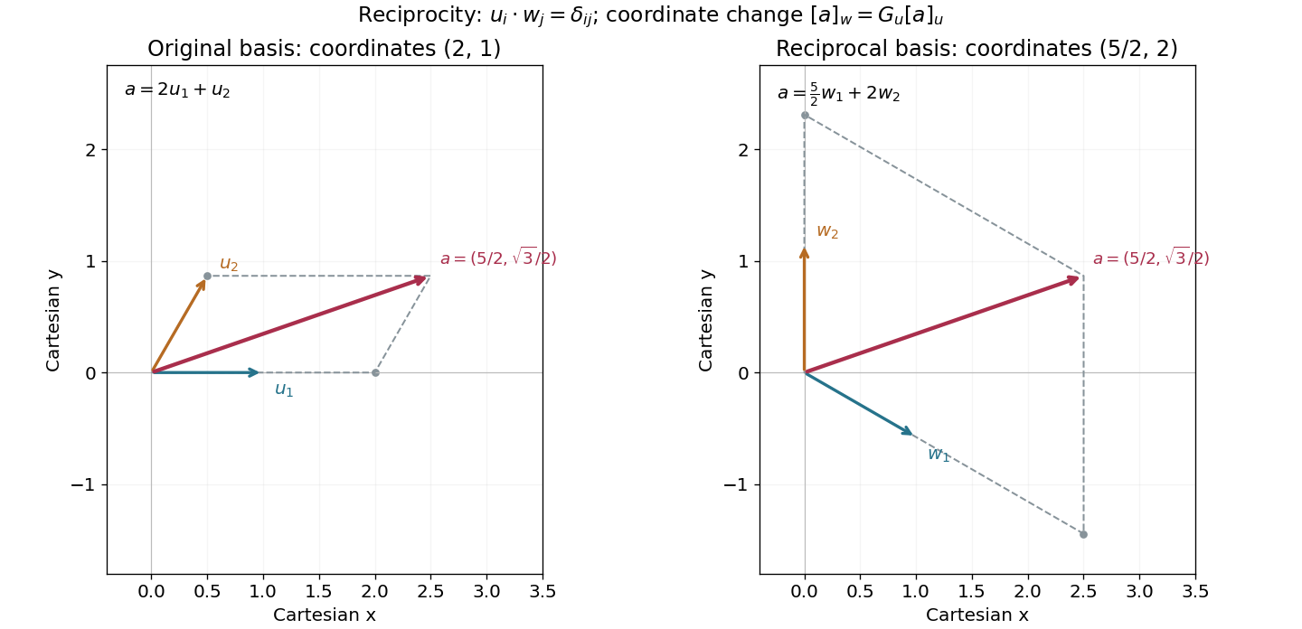
The two reciprocal bases satisfy . Expanding each vector in its specified basis and using real bilinearity givesThe simple sum-of-products formula holds because the two coordinate vectors use paired reciprocal bases. It does not require either basis to be orthogonal, and would generally fail if both sets of components were taken in the same nonorthogonal basis.
Take the inner product with in . The reciprocal basis condition gives . Expanding instead in the basis proves the reciprocal-basis coordinate transformationThus is the Gram matrix of the original basis. It is a positive-definite matrix, so this change of basis is invertible.
In the specified two-dimensional Cartesian frame,Solving the four dot product conditions givesThey are perpendicular to and , respectively, with lengths adjusted so the other dot product is one. Equating the Cartesian components of givesConsequentlywhich agrees entry by entry with the Gram matrix computed directly from the two unit basis vectors.


Articles by others on the same topic
There are currently no matching articles.