Source paper: Oxford source archive, member
2015/CP4_Sept_2015.pdf. The dated cover establishes the 10 September 2015 resit despite its generic Trinity Term heading. All four Section B options are treated.Start with the Maclaurin series . Put into the binomial series . Keeping terms through givessoSince and , term-by-term integration supplies the constant of integration and givesThe expansions hold near zero; the nearest real poles at limit their radius of convergence to . The derivative relation also independently checks all three displayed coefficients of the tangent function.
The Maclaurin series give and . Therefore , and cancellation of the common leading power givesThe argument applies from either side of zero: both leading terms involve the even power . The expression need not be defined at zero itself for its limit to exist.
Combine the two singular terms before taking the limit:For near zero, within the real domain , the Maclaurin series is . HenceThe two individual terms have divergent limits; their leading singularities cancel. Evaluating them separately as an “infinity minus infinity” subtraction would not justify the finite result.
Let . The trigonometric identity changes the expression to . Since ,The negative sign is also forced geometrically: near its maximum, is negative while the numerator is nonnegative. Both numerator and denominator vanish quadratically, so one application of a first-derivative argument alone would not yet resolve the indeterminate form.
Work on a domain with , and suppose is differentiable at . The multivariable chain rule givesMultiplying the first equation by and the second by cancels their common terms:The geometry is that stays fixed along a radial dilation . Thus is constant along each admissible radial ray, and the differential operator differentiates along that ray. This is the degree-zero case of Euler homogeneous function theorem. The displayed quotient does not define a function at without additional extension data.
The proposed linear change of variables makes the two pairs of boundary lines constant-coordinate lines: and . Thus the image of the parallelogram is the rectangle , .
The forward Jacobian matrix and its determinant areInverting gives , , so the area element is . The absolute inverse Jacobian determinant, rather than the forward determinant, belongs in the transformed area integral. Consequentlywhich yields . The transformed denominator is bounded below by one throughout the region, so no singular or improper integral is involved.
For a twice continuously differentiable function , first check the stationary-point condition . Write its Hessian matrix as , with , and . The second-derivative test uses : if and , the point is a strict local minimum; if and , it is a strict local maximum; if , it is a saddle point. If , the quadratic test is inconclusive and higher-order terms or a direct argument are needed.
For , the first derivatives vanish at the origin andThus . Directly, for nearby nonzero , while for nearby nonzero . The presence of both increasing and decreasing directions confirms the Hessian matrix classification.
Let and . Its partial derivatives areso both vanish at and . Evaluating the second derivatives at a point with givesTherefore the Hessian determinant is . Its two diagonal entries are negative at and positive at . HenceThese are also global extrema: for positive , the factor maximizes the positive value at , and differentiating fixes its positive maximum at . Oddness in supplies the corresponding global minimum.
The divergence theorem states that, for a sufficiently smooth vector field on a volume with piecewise smooth closed boundary ,Here is the outward unit normal. The left-hand side is the total outward flux; the right-hand side adds the local divergence throughout the volume. The orientation and the requirement to include the complete closed boundary are essential.
Read the given vector field as the three-dimensional field . Its divergence is the sum of the three matching-coordinate partial derivatives:The absence of a component does not make the three-dimensional flux vanish: the field still flows outward through surface normals with horizontal components.
The enclosed volume lies above and below . In cylindrical coordinates, its limits are , , , with volume element . The divergence theorem givesThus the volume is , and the outward flux is .
A direct check separates the boundary into its cap and base. On the base, . On the graph , the upward vector area element is , so the cap flux is , in agreement with the volume calculation.
For a real propagating positive-frequency branch, require and . If is the usual nonnegative cutoff, the source condition gives this branch. With an arbitrary real negative , that inequality alone is insufficient: and satisfy it but make the displayed square root imaginary.
On the positive-frequency real branch, the phase velocity givesDifferentiate the dispersion relation to obtain the group velocity:ThereforeFor and a nonzero cutoff, while ; when , both equal . The constant is the velocity scale in this assumed medium, and need not independently be identified with the vacuum speed of light. A group velocity describes a narrow-band wave packet on the chosen differentiable branch, rather than automatically fixing a signal front velocity in every dispersive model.
Embed the planar vector field as , independent of . Applying the Cartesian curl formula givesConsequently, for continuously differentiable components,This is the local closedness condition for the one-form . To infer global path independence from this condition alone, the domain also matters: it suffices that the planar domain is a simply connected space. The polynomial field in the next calculation is defined on the whole plane, so there is no missing-hole obstruction.
Set and . Their mixed derivatives agree: . Both components are smooth on all of , a simply connected space, so the line integral is path independent.
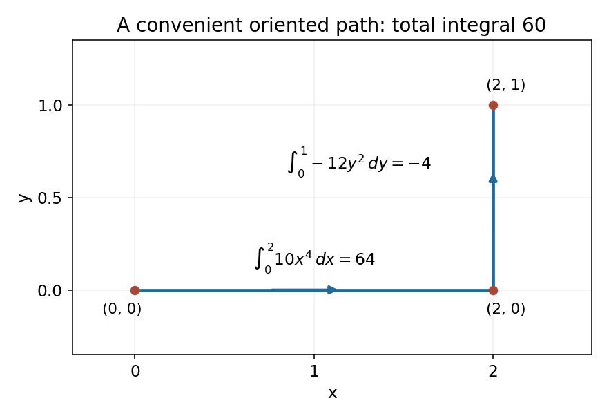
Choose a horizontal segment from to followed by a vertical segment to . On the first, and ; on the second, and . ThusThe selected path and its orientation are shown below. No contribution comes from a differential whose coordinate is held constant on a segment.
A one-form is an exact differential if a single-valued differentiable potential of a conservative vector field satisfies and on the domain. Then it equals , and its integral along a path is the endpoint difference of .
Integrate with respect to :Its derivative is . Matching the required second component forces , so the additive constant is arbitrary andThe fundamental theorem for line integrals now givesindependently of the convenient segmented path used before. Merely checking equality of mixed partial derivatives on an unspecified domain would not by itself construct this globally defined potential.
Take to be a simple closed, piecewise smooth curve oriented counterclockwise around its interior . Green's theorem applied to and givesThe orientation is essential: a clockwise unit circle gives , whereas twice its ordinary unsigned area is . For a nonsimple curve, the corresponding formula concerns signed area with winding multiplicity rather than one unsigned enclosed area.
The original diagram has three horizontal spans , and . In the small-slope approximation the massless string segments are straight and their transverse force components are tension times slope. The horizontal tension components cancel to first order.
For the first bead, the left segment contributes and the middle segment contributes . For the second bead, the middle contribution is and the driven right segment contributes . Newton's second law therefore givesWith and , the coupled equations of motion areThe factor two in the driving term follows from the right span having length , while the middle span has length . Treating all three spans as equal would change both the coupling and the normal mode frequencies.
The natural normal modes belong to the homogeneous system with both end displacements fixed at zero. Seek , soThe characteristic polynomial is . The eigenvectors and therefore giveThe symmetric mode leaves the middle segment horizontal, while the antisymmetric mode bends it strongly and has the higher restoring stiffness. Defining and diagonalizes the driven equations too:This shows that the boundary drive excites both natural modes; neither natural resonance is removed by a zero drive projection.
Away from the natural resonances, seek a periodic particular solution . Let . The amplitude equations areTheir determinant is , giving the signed displacement amplitudesA negative sign denotes a phase reversal relative to the prescribed cosine; physical amplitude magnitudes are . In the quasistatic limit,These are the values of a straight string interpolating between endpoint displacements and at bead positions and along a total length .
Because damping is explicitly absent, this periodic response is not a unique attracting late-time state. Arbitrary homogeneous oscillations at and persist unless the initial conditions eliminate them. At either natural resonance, the drive produces secular growth rather than a finite bounded periodic response. Thus “steady state” here refers to the selected particular solution away from the poles.
At , , so the periodic amplitudes becomeThe second bead is stationary in this particular motion, although the endpoint oscillates. The first bead moves at twice the endpoint amplitude and in opposite phase. This is an antiresonance of the second-bead response, not a natural resonance of the complete two-bead system.
The force balance makes the cancellation explicit. At , the middle segment supplies transverse force , while the end segment supplies ; these cancel on the second bead. The first bead then oscillates between two effectively fixed neighbours with restoring coefficient , whose single-coordinate natural angular frequency is .
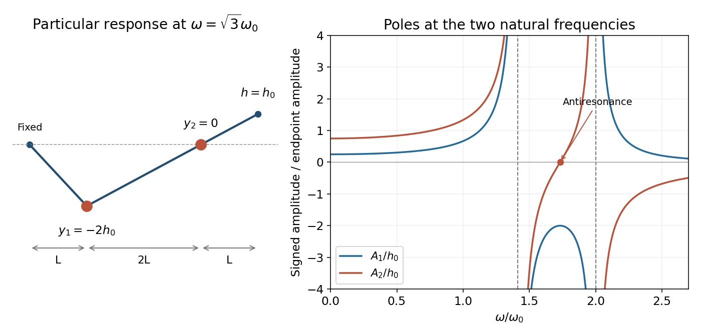
Periodic bead responses and the stationary second bead at antiresonance
. Details. As elsewhere in the undamped problem, this exact nodal motion presumes initial conditions selecting the periodic particular response. Additional free normal modes would move the second bead as well; they do not decay automatically.
Let a differentiable curve lie on the level surface , and pass through the point under consideration. Differentiating the constant relation along the curve givesEvery surface tangent vector arises as the velocity of such a surface curve, so the gradient is orthogonal to every tangent direction. At a regular point, where , it therefore defines a normal direction, with unit normalIf , the dot-product identity is still true but the zero vector does not determine a normal direction; a regularity hypothesis or another defining function is needed. For example, defines the plane at level zero but has vanishing gradient everywhere on that plane.
Write the fixed point as and the variable point as . Then andSince the fixed point is not on the surface, at every point being considered. Componentwise differentiation gives , henceThus the gradient points from the fixed point towards the variable point and is a unit vector. Keeping the fixed point fixed is important: differentiating a distance between two simultaneously moving points would include both endpoint derivatives.
Let , , and define the outward-from-focus unit vectors and . The ellipse is the nondegenerate level curve , with . The previous gradient result givesIf is a unit tangent at , orthogonality to the level-curve gradient impliesTherefore . These absolute dot products are the cosines of the acute angles made by the two focal lines with the unoriented tangent line. Thus those angles are equal.
Equivalently, the outward unit normal is , the bisector of the two unit focal directions. Its denominator is nonzero for a nondegenerate ellipse. Using , the specular reflection formula becomesThis algebra proves the equal-angle statement with the incident and reflected ray directions correctly oriented, rather than confusing the line with the outgoing direction .
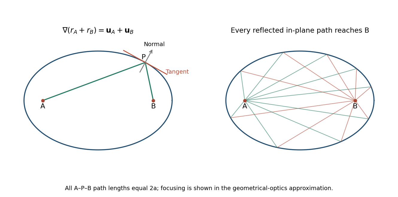
A ray leaving focus and reaching a boundary point has incoming unit direction . By the law of reflection, its normal component reverses and its tangential component stays fixed. The result just derived shows that the reflected direction is , pointing exactly from to focus . Thus all such in-plane rays from one focus converge to the other after one reflection, in the ideal geometrical optics model.
Moreover, every reflected path has the same total length . In a uniform medium their propagation times are equal as well, so different reflection points do not introduce a geometrical path-length spread. Finite wavelength, surface errors and incomplete reflecting coverage limit a real focus; the ideal argument concerns rays in the plane of the ellipse. It does not assert that an arbitrary three-dimensional surface with only one elliptical section focuses every out-of-plane ray.
Consider a string element of equilibrium length . Its mass is , where is mass per unit length. Under the small-slope approximation, the tension is approximately uniform and its transverse component at an endpoint is . The two endpoint forces have net transverse componentNewton's second law gives . Cancelling the element length yieldsThis is the one-dimensional wave equation for transverse displacement. Its derivation neglects gravity, bending stiffness and nonlinear changes in tension and segment length; the given small slope makes those omissions consistent to first order in the displacement.
Seek a separated normal mode . Substitution in the wave equation gives . For an oscillatory mode choose the separation constant :The fixed endpoints impose . In , the first condition gives , and the second requires . Nonzero displacement therefore requiresEach spatial shape has fixed nodes and an oscillating overall amplitude: a standing wave. A general lossless motion is a superposition of these standing normal modes, not necessarily one single-frequency standing wave. The solution is trivial under both fixed-end conditions and does not supply an additional vibrational mode.
Use with . The initial shape becomesThe sine functions are orthogonal on , so this decomposition directly identifies the two nonzero spatial normal mode coefficients. Since the string is released from rest, every time-dependent sine coefficient vanishes and the subsequent motion isThus the signed mode amplitudes are , and for ; their magnitude amplitudes are and . The factor of two in the second angular frequency is fixed by the same boundary conditions as its spatial wavelength.
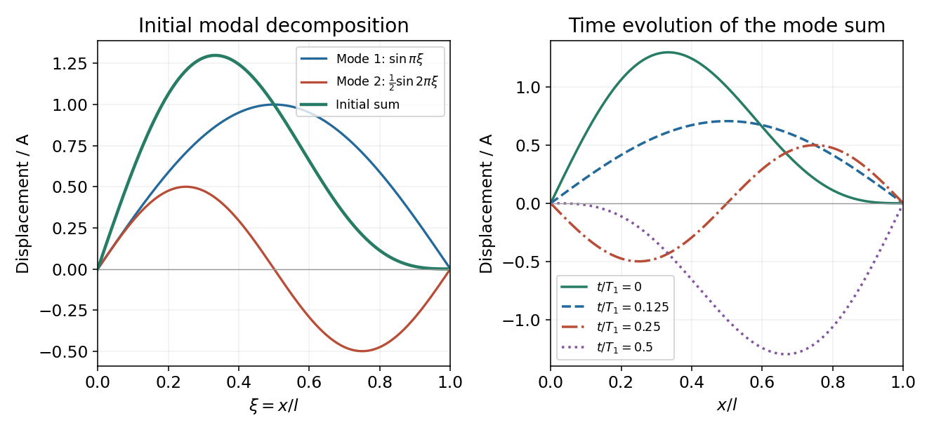


For a single normal mode , the kinetic energy is the integral of . Using givesThe extra string length is . Multiplying by tension gives the quadratic potential energy, so impliesSince , the sum is time independent:For the released shape, and , soThe second mode's smaller displacement is offset by its doubled spatial wavenumber and angular frequency. orthogonality of distinct sine and cosine spatial modes eliminates cross terms in the integrated energies, so the total is their sum. Initially the kinetic energy is zero and all the energy is stored in the string's deformation; during the motion the total remains constant.
Articles by others on the same topic
There are currently no matching articles.