This University of Oxford Part C paper combines Mathematics and the Environment in section A with Mathematical Physiology in section B. [ref]
https://www.whatdotheyknow.com/request/maths_past_papers_3. Source release
The archive preserves the complete editable seven-page paper. Bounded searches of official sources found no advertised answers for this exact paper. The solutions distinguish linear and asymptotic conclusions from exact nonlinear claims, and identify the carrier-total typo and small-parameter respiratory approximations.For Röthlisberger channel drainage, is the water-filled cross-sectional area of the subglacial channel, its volume discharge, the mass of ice melted per unit channel length per unit time, and the effective pressure, namely ice overburden pressure minus water pressure. The first balance converts melt mass to area growth through division by ice density , and subtracts material creep closure . The cubic pressure dependence comes from the adopted ice-flow law; includes its material and geometric factors.
The second relation balances the downslope hydraulic driving gradient against the adopted frictional pressure loss. It is an instantaneous discharge-area law, giving for positive downstream flow. The final balance equates latent heat needed to melt the channel walls with the gravitational power dissipated per unit length, . It assumes that this dissipated power is available for melting rather than substantial sensible heating or other energy losses. The model thus couples melt opening, pressure-driven material creep closure and hydraulic discharge.
With constant lake surface area, raising its level by changes its volume by . The symbol in the proposed balance is an effective filling rate measured as lake-level rise per unit time, so the volume inflow is . Volume conservation givesThus the lake rises when its inflow exceeds channel discharge and falls in the opposite case. If an inflow were instead specified directly as a volume rate , its contribution would be ; keeping these units distinct is necessary for the interpretation of .
Hydrostatic pressure at the entrance is , with a constant reference pressure. Therefore , and constant overburden pressure givesA filling lake raises water pressure and lowers effective pressure, reducing material creep closure. A draining lake has the reverse effect. These signs supply the pressure feedback in the coupled drainage model.
Write dimensional variables as their scales times dimensionless variables, with positive scales . For compactness defineA consistent explicit choice isThese identities give , , and . Substitution therefore leaves the unit coefficients in all four balances, and the sole supply parameter is . Expanding its scales yieldsAfter dropping scale hats, eliminate the instantaneous quantities to obtain the useful two-dimensional systemThese scales assume a positive slope, positive friction coefficient and nonzero lake area; they nondimensionalize exactly the hydraulic law printed in the source.
For , the positive equilibrium isSet and and retain first-order terms. The linear system isDifferentiating its first row and using the second givesIn particular the trace is positive and determinant is . The steady drainage state is linearly unstable for every positive supply, whether its instability is oscillatory or nonoscillatory.
The characteristic roots satisfyThey are a nonreal conjugate pair precisely when , or . ThereforeIn lake-coupled Röthlisberger drainage instability, above this value the real part is , so nonzero linear perturbations are sinusoidal oscillations with an exponentially growing envelope. Their angular frequency is .
Physically the feedback represents repeated lake filling and pressure increase, channel enlargement by melting, rapid drainage, pressure reduction and material creep closure. Large drainage events are glacial lake outburst floods, or jökulhlaups. The unbounded amplitude is a conclusion of the linearized equations, not a proof of infinite physical discharge or an indefinitely growing nonlinear solution. Once perturbations are comparable with the equilibrium scales, nonlinear dynamics and constraints such as lake depletion must be retained. At the threshold the two real roots coincide; below it the instability is nonoscillatory.
The cross-sectional area multiplied by the mean downstream speed is the volume flux . The term is local storage change per unit river length, is net downstream export per unit length, and is lateral volume input per unit length per unit time, for example distributed tributary or runoff supply.
For a fixed reach , incompressibility and constant density giveApply the fundamental theorem of calculus and localize the resulting integral identity to obtain . The density cancels because every term transports the same water; no sediment source is included in this balance.
To obtain a power-law river kinematic wave, let be the wetted perimeter and the small bed slope. A uniform-flow force balance per unit river length is . With a Chézy friction law , it gives . Thus the hydraulic radius determines the power of area.
For a channel family with , where , we have , with . Set and . ThenFor example a broad fixed-width rectangular channel has approximately constant wetted perimeter, giving ; a geometrically similar channel family has , giving . The exponent is therefore a geometry-dependent consequence of the friction balance, not a universal arbitrary value fixed by Chezy's law alone.
At equilibrium , so for an upstream boundary flux . HenceWithout a specified upstream condition this integration constant must be retained. On a region of positive area, the characteristic speed is , increasing downstream along the equilibrium. Small disturbances move downstream, spread in space as this speed increases, and decrease in area amplitude in the manner derived next. They are transported away from a fixed location; the model has no diffusion giving instantaneous smoothing. Finite-amplitude compressive disturbances can steepen into shocks because the flux is convex, , so the small-disturbance picture is not a global no-shock assertion.
Taylor expansion gives . Subtract the equilibrium equation and write to obtain . Set . Since is time independent, . The travel coordinate for a conservative transport perturbation transforms this into , and thereforeThe conserved quantity along a characteristic is the flux perturbation , explaining the diminishing area amplitude as grows.
Differentiate the equilibrium relation to get . Thus the arrival time is explicitlyFor zero upstream flux the integral remains finite, giving the limiting formula with its second term zero. However then makes the displayed amplitude formula singular at the head; a uniformly small arbitrary area disturbance imposed exactly there is outside this linearization. A positive upstream flux avoids that degeneracy.
Here is water depth, the depth-averaged downstream speed, bed elevation relative to the reference slope, and free-surface elevation relative to that reference. The constants are water and grain densities, is the reference bed slope, bed shear stress, bed porosity, suspended sediment mass concentration, bedload solid volume flux per unit width, and erosion and deposition velocities. The settling speed is denoted by in the constitutive laws.
Depth integration of incompressible water conservation gives the depth-storage plus discharge-divergence balance. Depth-averaged momentum has local and advective acceleration on the left, and gravity driven by the actual surface gradient together with bed drag on the right. Hydrostatic pressure and a shallow-water approximation underlie this Saint-Venant description.
Suspended sediment conservation first has the conservative form ; the water balance reduces it to the material-derivative form printed in the source. Solid bed volume per unit horizontal area is . Its storage plus bedload divergence equals deposition minus erosion, giving the Exner bed balance. Adding the suspended and bed balances after converting bed volume to grain mass cancels exchange terms: erosion and deposition transfer sediment between the two reservoirs rather than create it.
Take an arbitrary reference depth , and select so the uniform reference flow balances drag and slope. Work with positive downstream velocity, so in the dimensional constitutive laws. Introduce the erosion and bedload scalesMatching erosion with deposition, suspended advection with erosion, and bed storage with erosion gives respectivelyUse for the scales of and too, so survives unchanged. After dividing the balances by their matched scales, the parameters areFor example the momentum balance divided by has inertial prefactor , surface-gradient term , and equal slope/drag prefactors , because . The suspended balance has source , and the bed balance has its negative with unit bed-time coefficient by the definition of . These substitutions give the entire stated dimensionless system; is dimensionless bedload, with its dimensional scale already absorbed into .
For quasistatic bed stability with suspended sediment, in the leading approximation, and . For spatially varying perturbations at fixed unit water flux and fixed surface level, write , , , . The constraints give and . Linearizing the suspended and bed equations yieldsFor a Fourier mode , the first relation gives ; substitution into the second givesThus every nonzero spatial frequency has negative growth rate, independently of . The parameter changes propagation, not damping. The spatially uniform mode has and is neutral, representing a change among uniform reference states compatible with the leading constraints. Hence there is no growing linear mode in this approximation; the claim is stability, not strict decay of every homogeneous perturbation. Restoring the small discarded terms or changing boundary conditions requires a separate calculation.
In alternating-access carrier transport, the four reversible reaction pairs are , , and . Binding and unbinding use ; both conformational pairs use in each direction. Define the net binding rates and . Mass action and the change of each species in each reaction giveFor example binding consumes one free interior substrate and one free interior carrier, and produces one interior complex; loaded-carrier transformation then moves that bound substrate across the membrane. A bare-carrier transformation alone does not transport substrate. The concentration convention implicitly uses compatible compartment-volume normalization, as required for the stated unweighted conservation laws.
Adding the two complex and two free-carrier equations cancels binding and conformational exchange, givingEach free or bound carrier contains one carrier protein, and the model neither synthesizes nor degrades it. Adding the two free-substrate and two bound-substrate equations likewise givesBinding stores substrate temporarily and loaded conformational exchange relocates it; neither changes total substrate. The two invariants count distinct conserved chemical moieties. The constants and should not be interchanged: protein and substrate need not be present in equal amounts.
Replace only the free-substrate equations byThe other four equations remain as above. The carrier invariant remains unchanged because no protein is added or removed. The two external substrate terms cancel in the total-substrate balance, so the second invariant also remains unchanged. This cancellation describes a balanced source and sink, even though there is a nonzero throughput. A constant sink is physically meaningful only while substrate concentrations remain nonnegative; it is not a state-dependent removal law valid after an interior reservoir is exhausted.
At steady state the interior free-substrate balance gives . Substituting this into the interior free-carrier balance gives . ThereforeFor positive inward throughput there are more free carriers facing inward: release of transported substrate must be followed by outward return of empty carriers at net rate .
The relation means . Put and substitute the preceding expression for :The first term is the equilibrium binding contribution from the outward free-carrier pool; the additional terms account for the maintained current and the excess inward-facing free carriers. This is a steady throughput relation, not a detailed-balance assumption.
The exterior free-substrate equation gives at steady state. Thus , andThe sign of the current term is opposite to the interior relation because substrate is supplied to the exterior and removed from the interior. Nonnegative occupancies are selected by the complete steady transport solution and compatible substrate totals.
The loaded-carrier balance gives . Substitute the preceding two complex concentrations and collect the current terms:Next carrier conservation givesEliminate between these relations and set . Simplification yieldsHere must be the total carrier protein, as in the conservation equation. Calling it total substrate in the final line of the scan is a typographical inconsistency; total substrate is the different invariant .
For carrier-turnover saturation of passive transport at fixed , write , and . Then , soThe flux is outward when the substrate gradient is reversed and inward when . Saturation occurs because there is a finite carrier population and finite binding-release/conformational turnover: arbitrarily abundant exterior substrate cannot make carriers cycle arbitrarily quickly. This is passive facilitated transport, so no maintained flux remains when the two free concentrations agree. Varying at fixed compares reservoir-controlled steady states or systems with different total substrate; it is not a trajectory preserving one fixed .
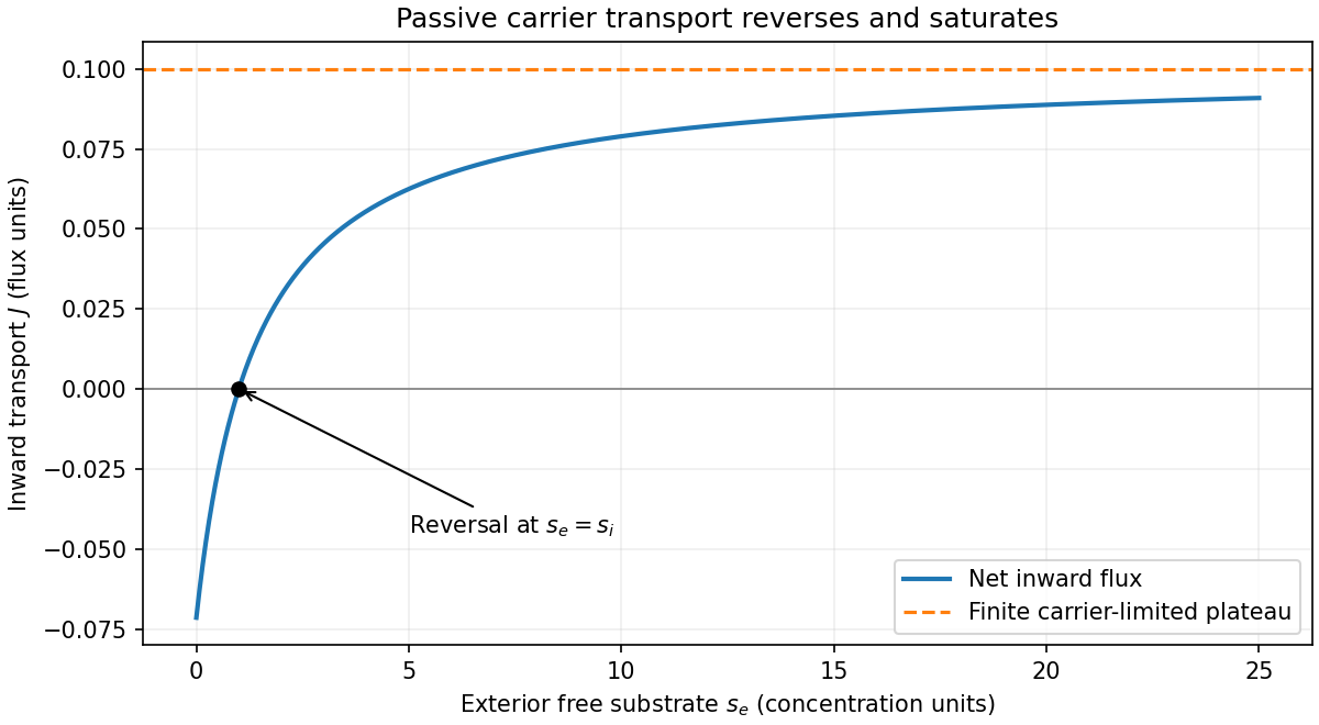
Carrier-mediated transport: reversal and saturation at fixed interior concentration
. Details. The cytoplasmic concentration gains a constant influx from outside the cell and loses calcium through a first-order extrusion term . The pump flux moves calcium from cytoplasm into the sarcoplasmic reticulum, saturating with cytoplasmic concentration through a Hill function with scale , maximal rate and exponent . The release flux returns stored calcium to the cytoplasm. It requires both calcium in the store and calcium-dependent activation of release; its two saturating factors have scales and exponents . This represents calcium-induced calcium release. The leak is passive return from the store.
Every internal transfer appears with opposite signs in the two balances, so in the model's compatible volume normalization. Only influx and extrusion change the total. The nonlinear pump and activated release can redistribute this total rapidly and generate oscillations even with constant external input.
For the three-region calcium nullcline, defineFor , , as , and . Thus there is exactly one positive root for every positive . The curve starts at the origin and initially satisfies .
On the large- branch away from the crossing, replace by one. This gives where this is large and positive. Near retain the next term and linearize :Finally where the leak is negligible compared with the other terms, , so on the side . These are overlapping asymptotic descriptions with different validity ranges, not three exact disconnected curves. The curve rises to a large peak, falls sharply near , then approaches a small finite level as . At leading small- order that last level is .
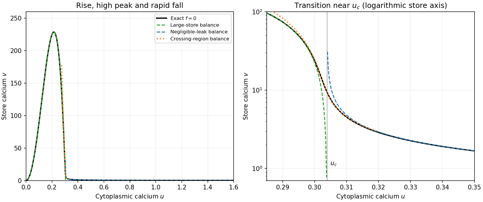
At every equilibrium the store balance gives , and adding times that balance to the cytoplasmic one gives . The unique-root result therefore gives a single positive equilibrium . Its Jacobian iswith derivatives evaluated at that equilibrium. At small , and the trace is negative; sufficiently large also has , since is of order and of order . Thus both extreme regimes have a linearly stable unique equilibrium.
The fast variable is not alone. Using total-calcium fast fibres, introduce total scaled calcium . Then , while on fast time the leading equations give , and constant. Fast paths are therefore straight lines of slope in the plane. Attracting portions of the critical manifold satisfy , rather than merely . Along , slow motion obeysStarting with large and , drives a rapid move upward and left, loading the store until the trajectory approaches the right attracting branch. For large in the right stable regime, slow motion on that branch carries it toward ; the direction reverses appropriately if the starting value lies below that equilibrium. For sufficiently small , slow motion travels left along the right branch until its fold, then a fast approximately constant- jump carries the trajectory to the left attracting branch. Subsequent slow motion reaches the small- equilibrium. At a fold the slow approximation is singular, so the full equations resolve the transition. At very small an additional loss of time-scale separation is possible because the rates themselves vanish; the fast/slow drawing describes the separated portions, not a uniform estimate arbitrarily near the origin.
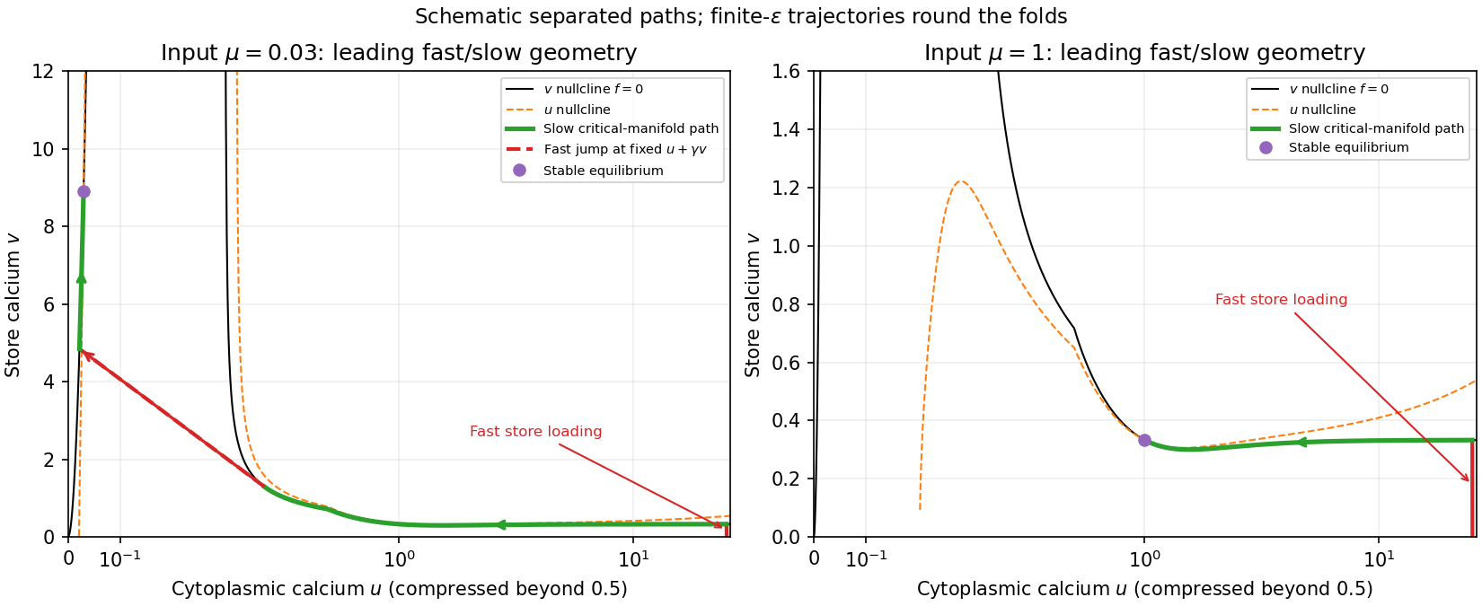
For Hopf thresholds in a two-pool calcium model, with the unique equilibrium parametrized by , locate changes of stability by solving the two equationsIf there are two simple roots with positive trace between them, the equilibrium is a repeller throughout that interval, since its determinant stays positive. At a nondegenerate crossing a Hopf bifurcation is possible, with linear frequency . A complete classification of criticality requires a nonlinear coefficient, not merely the trace calculation. At leading singular order the thresholds approach the folds determined by and , equivalently .
Periodic solutions are also supported globally in the positive quadrant. The axes point inward for positive input, bounds , and the equation then bounds by a linear restoring term plus a bounded source. A large rectangle can thus be chosen forward invariant. For an initial point distinct from the repelling unique equilibrium, its omega-limit set cannot contain that equilibrium or a boundary equilibrium. The Poincaré-Bendixson theorem supplies a periodic orbit. In the strong separation regime it follows the two attracting branches and jumps between them, a relaxation oscillation.
The interval requires the maximum of along the critical manifold to exceed ; the listed scale hierarchy alone is not a substitute for that test for arbitrary remaining constants. As an explicit example, , , and give approximately and . At the trace is positive, whereas at and it is negative. The figures use this example and label their singular-limit portions accordingly.
In a relaxation cycle, cytoplasmic calcium rises slowly on the left attracting branch while total calcium is accumulated, then rises rapidly during store discharge along a constant- fast path to the right branch. It subsequently decreases on the right slow branch as extrusion dominates input, and finally drops rapidly during store uptake back to the left branch. The result is a repeated pulse with slow sections joined by sharp transitions, rather than a sinusoid except near a small-amplitude Hopf bifurcation.
For explicit time labelling, the compatible scaling , gives , , , , and . Hence an interval corresponds to physical duration . Slow-branch times can be computed by integratingin the direction of motion; fast-jump durations are omitted at leading order. The plot uses that quadrature, with vertical lines representing the limiting rapid transitions. Finite rounds those lines and changes the precise amplitude and period, especially near folds.
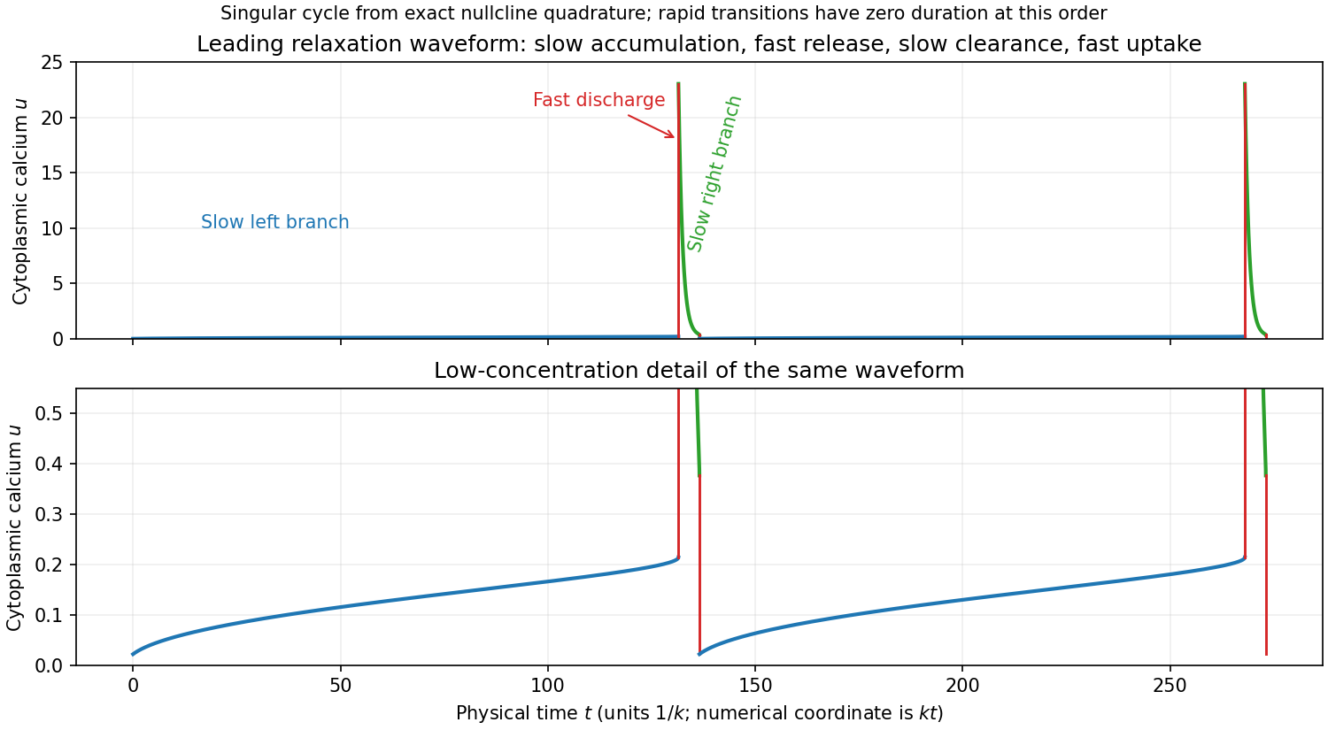
Leading relaxation waveform of cytoplasmic calcium, with physical time measured in inverse-extrusion-rate units
. Details. In delayed carbon-dioxide ventilation feedback, is the effective carbon-dioxide partial pressure of the lumped body compartment. Its stored carbon-dioxide amount is proportional to , with effective capacitance , so is its accumulation rate. Metabolism produces carbon dioxide at rate . Ventilation removes it at a rate proportional to partial pressure times ventilation, , with gas-conversion constants absorbed into the model coefficients. The equation is therefore a one-compartment carbon-dioxide balance: production minus respiratory removal equals accumulation. It idealizes mixing and treats metabolic production as constant over the time scale of interest.
Chemoreceptors respond to carbon-dioxide levels, but feedback is delayed by blood transport to sensing sites, neural processing and the response of respiratory muscles. A fixed positive delay approximates their combined effect. The ventilation at the present instant therefore depends on the earlier pressure, , not just on . This delayed negative feedback can overcorrect after the pressure has already changed, providing a mechanism for oscillatory breathing. The delay equation requires a pressure history over an interval of length , rather than a single initial value.
The positive-part law is a threshold-linear approximation to the ventilatory response. Below the apnoeic threshold , this model assigns zero ventilation; above it, each pressure increment produces a proportional ventilation increase, with gain . Taking the positive part ensures a nonnegative ventilation rate rather than the unphysical negative rate that unrestricted linear extrapolation would give. It is a local idealization of the response, not a claim that actual physiology lacks other respiratory drives or saturates nowhere. In the delayed model this response is evaluated at the delayed pressure.
Distinguish physical time from scaled time . PutThen , givingA steady state must be positive, since otherwise ventilation vanishes while production remains positive. It solves , soThe value printed in the question agrees only through first order. Thus it is a small- approximation with error of order , not an exact equilibrium for nonzero . The other quadratic root is negative and inadmissible for this steady ventilation balance.
Since the steady state is strictly positive, the positive-part function is differentiable in a neighbourhood of it. Write . Retaining first-order terms givesSubstitute the exponential mode to obtainHere the last equality uses the exact steady-state equation. For small , and . Linearizing at the exact root avoids carrying a spurious constant residual from the printed approximate equilibrium.
For real , draw and . The first is nonnegative and increasing, while the second is negative and approaches zero from below. They cannot intersect on the nonnegative real axis. At zero the characteristic function equals , so a stationary zero-root crossing is excluded as well.
Consequently a loss of stability from a stable regime cannot occur by a real eigenvalue crossing through zero. It must involve a conjugate pair crossing the imaginary axis at nonzero frequency, yielding oscillatory instability. This does not mean that every characteristic root is nonreal: negative real roots may exist and are harmless for stability. The graph and imaginary-axis conditions are shown together below.
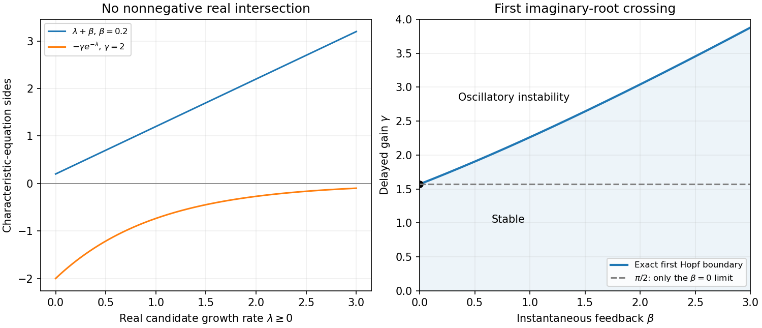


For the first Hopf boundary of scalar delayed negative feedback, first, if a root has nonnegative real part then . For this is impossible, apart from the potential equality case , already excluded. Thus is necessary for instability, although not sufficient by itself.
At an imaginary root with , separate real and imaginary parts:The first crossing uses for , and satisfiesThe period is in scaled time; its physical value is . Higher-frequency branches have larger critical gains. For fixed , stability at zero delayed gain and absence of any earlier imaginary or zero-root crossing identify this lowest branch as the first stability boundary. Its crossing is transverse: implicit differentiation of gives at the imaginary rootFor very small , , so and . Therefore is exact in the limit and is the leading approximation for small positive . At that limit first has an imaginary pair at ; subsequent pairs occur at and cannot be the first loss of stability. A nonlinear Hopf theorem, including its nondegeneracy conditions, is needed to turn the linear imaginary mode into a claim about a particular finite-amplitude periodic branch.
Articles by others on the same topic
There are currently no matching articles.