Since , we have and . Its multiplicative order therefore divides the prime number . It cannot be one, because . Thus the order is exactly .
To find the desired prime divisor, use the cyclotomic polynomialChoose a prime factor of this integer. Since , we have , so . Also . If , then , contradicting . Consequently has multiplicative order in the multiplicative group of a finite field . Lagrange theorem givesThis divides as required. Notice that order modulo a composite integer alone would not justify selecting an arbitrary prime divisor; the cyclotomic polynomial selects a suitable one.
If there were only finitely many such primes , choose , with the empty product interpreted as one. Each divides and hence does not divide . The preceding argument supplies a further prime dividing that integer, a contradiction. There are infinitely many primes in this residue class.
Here is a direct Chebyshev alternation theorem argument proving optimality, without assuming the theorem. At the five ordered pointsthe error takes the alternating values . If a polynomial of degree at most three had strictly smaller uniform error, then would have alternating strictly positive and strictly negative values at these points. The intermediate value theorem would give a distinct root in each of the four intervening intervals. A nonzero polynomial of degree at most three cannot have four distinct roots. This contradiction proves the required minimax inequality.
There are two conventions for loxodromic Möbius transformations. In the inclusive convention, a transformation conjugate to with is loxodromic, including a hyperbolic Möbius transformation with . Under that convention the assertion about discs is false: preserves the upper half-plane, and a Cayley conjugation gives an invariant ordinary disc.
The question uses the classification in which hyperbolic Möbius transformations and genuinely spiralling loxodromic Möbius transformations are separate. Thus here the multiplier satisfies and . Such a Möbius transformation has two distinct fixed points; after sending them to zero and infinity it acts by the stated dilation and rotation.
For a determinant-one representative, put . Its eigenvalues are , with , and the normalized multiplier is or its reciprocal. If is real, the eigenvalues are either real or conjugate unit-modulus numbers. These give the hyperbolic, elliptic, parabolic or identity cases, not a genuine spiral. Conversely, a real eigenvalue or a unit-modulus eigenvalue makes real. Hence the practical criterion in the question's convention isChanging the determinant-one representative by its sign does not affect this criterion.
Finally, conjugate an invariant disc to the upper half-plane. A Möbius transformation preserving that half-plane has a representative in : preservation of the boundary gives real coefficients up to a common scalar, and preservation of the chosen side makes the real determinant positive, allowing normalization to one. Its trace is real. Trace is invariant under conjugacy, up to the harmless sign of the representative, so a disc-preserving transformation cannot be genuinely loxodromic. This proves the intended assertion while specifying its necessary terminology.
In a specified finite cyclic group , the discrete logarithm problem is to recover modulo from and . A common choice is a large prime-order subgroup of a multiplicative group of a finite field.
For Diffie-Hellman key exchange, Alice and Bob independently choose private exponents , transmit , and compute respectively and . Both obtainSolving a discrete logarithm problem reveals a private exponent and breaks this exchange. The converse implication is not known in general: recovering from is the computational Diffie–Hellman problem, rather than literally the same task as computing a logarithm.
The advantage is that parties without an already shared secret can establish a fresh session key, which can then be used with efficient symmetric encryption. A classical secret-key system requires an earlier secure key distribution; ordinary public-key encryption can instead transmit a chosen key, but ephemeral Diffie-Hellman key exchange also permits forward secrecy when private session exponents are erased and the exchange is authenticated. Authentication is essential: an unauthenticated exchange is vulnerable to a man-in-the-middle attack.
For multilateral Diffie-Hellman key exchange with participants with private exponents , send tokens clockwise around a ring. Participant starts the token and sends it to participant . On each subsequent receipt, the receiver raises the token to their own private exponent and sends it onwards, until that token has made transmissions and reaches participant . Its exponent then contains every exponent except . The receiver raises it to locally, obtainingEvery participant receives one such final token. There are tokens with exactly transmitted group elements per token, giving transmissions. No private exponent is transmitted.
Write and fit the normal linear modelThe basic linear regression analysis assumes centered independent normal random variables of a common variance , conditional on the predictors. Independence between makes does not by itself establish independence between different models of the same make; that stronger assumption should be checked, or within-make dependence modelled. The requested R fit is
fit <- lm(log(price) ~ mpg + psngr + length + width + weight, data = cars)The estimate column contains the ordinary least squares coefficients. The standard error estimates the standard deviation of each coefficient estimator. The t value is its estimate divided by its standard error. The last column gives the two-sided p-value for a zero coefficient, using a Student t-distribution with residual degrees of freedom under the stated normal linear model; the stars summarize significance thresholds.
Conditional on the other predictors, passenger capacity and width have negative fitted coefficients, while length and weight have positive ones. All four are significant at the conventional 5% level; length is borderline. There is little evidence for an additional mpg effect once the others are included. These are conditional associations, not causal claims. For example, increasing weight by 100 pounds multiplies the fitted price by approximately , about 1.087.
A reasonable candidate simplification removes mpg and compares the nested models by an F-test, rather than treating a nonsignificant coefficient as proof of no effect:
fit2 <- update(fit, . ~ . - mpg)
anova(fit2, fit)
Inspect regression residuals, normal quantiles, residual-versus-fitted plots, leverage and influential observations. The correlated size predictors may produce multicollinearity; missing make effects, nonlinear terms or unequal residual variances may also matter. A random make effect or a covariance adjustment addresses the possible dependence noted above.
Put . The linearization at the zero solution isThe appropriate Fourier sine series isOrthogonality of the modes givesThus each mode grows or decays exponentially with its own eigenvalue, and the largest growth rate is the value. Strict linear stability analysis, meaning decay of every mode, is equivalent toAt equality the first mode is neutral in the linearization; the nonlinear terms decide its subsequent behavior. Above this length the first mode grows, giving linear instability.
A useful version of the Poincaré-Bendixson theorem says that a forward orbit of a continuously differentiable planar autonomous vector field which stays in a compact set has a nonempty compact omega-limit set; if that omega-limit set contains no equilibrium, it is a periodic orbit.
Let . Direct calculation givesFor , , so . In particular there is no equilibrium away from the origin.
On , both coefficients in the radial expression are strictly positive, so the flow crosses outward. On , both are strictly negative, so the flow crosses inward. Consequently the compact annulusis forward invariant. Any orbit starting there stays there, and its omega-limit set avoids the only equilibrium, the origin. The Poincaré-Bendixson theorem therefore supplies at least one periodic orbit in this annulus.
Choose on the right semicircle, with the continuous branch . ThenHere the integral is along that semicircle. Since , the pole lies outside the unit disc and the geometric series converges uniformly on the contour.
PutThe Euler integral for the hypergeometric function, initially for , givesThe prefactor follows from . Hence an antiderivative of the contour integrand before multiplication by isEvaluating at the endpoints with the chosen branch yieldsThis is first obtained where the individual expressions are defined. The original finite-interval integral is entire in , so analytic continuation gives the result elsewhere, taking removable limits at the apparent exceptional negative integers. That convention matters: the two separate hypergeometric terms may be singular even though their combination is finite.
For an autonomous Lagrangian, the canonical momentum and energy areAlong a solution of the Euler-Lagrange equation,The absence of explicit time dependence is essential to this conservation law.
The classical action is . If the final endpoint is moved along one fixed classical trajectory, while the initial endpoint is held fixed, the fundamental theorem of calculus givesThis total derivative is different from the partial derivative with fixed final position.
For a family of nearby classical trajectories, integration by parts gives the endpoint variationTo obtain the final term, the endpoint change in the variation at fixed parameter time is , while the changing upper integration limit contributes . The interior integral vanishes by the Euler-Lagrange equation. Therefore, on any smooth branch of classical boundary-value solutions,The chain rule along the endpoint trajectory now reads , consistently with the direct calculation.
The Jeans wavenumber in physical coordinates is . With wavelength defined as , the Jeans length isPressure opposes gravitational growth on physical wavelengths shorter than this; on longer wavelengths the gravitational term wins. Expansion also provides the damping term , so the actual growth is not generally the exponential growth of a static medium.
For the pressure-free, spatially flat matter solution, and the Friedmann equation gives . The perturbation equation becomesSubstituting gives . ThusThe growing mode scales as and permits the formation of structure; the decaying mode becomes negligible at late times. This is a linear result, valid while the density contrast remains small.
Write and associate the symmetric matrix . Define the left group action of by ; using instead describes the same equivalence classes. The transformed matrix is , so its determinant is unchanged. Hence the discriminant of a binary quadratic formis invariant under proper equivalence of binary quadratic forms.
A proper representation here means with . Such a vector extends to the first column of an integer determinant-one matrix by Bezout identity. After that change of variables the form has leading coefficient , and discriminant , so its middle coefficient satisfies . Conversely, such a congruence gives the positive definite integral formwhich represents at . It is primitive: a common divisor of all three coefficients would have its square dividing the squarefree discriminant 35.
For clarity, enumerate all the proper equivalence classes at this discriminant. Substitutions first arrange ; if , the determinant-one substitution makes the leading coefficient smaller. Repeating terminates because this coefficient is a positive integer. Thus every class has a reduced representative with . From it follows that , giving . Checking , with odd, yieldsThe two signs in the first pair are equivalent by replacing with , and in the second pair by the determinant-one swap. Thus the two forms in the question exhaust the classes.
The primitive representation criterion at discriminant minus thirty-five now follows. For odd prime to 35, the congruence modulo is solvable exactly when is a square modulo every prime divisor of . Necessity is immediate. For sufficiency, a nonzero root modulo each odd prime lifts to all required prime powers because its derivative is invertible; combine the lifts by the Chinese remainder theorem, also imposing . This gives the modulus-four condition since . We concludeBy quadratic reciprocity, the symbol equals . In particular each prime divisor must be a quadratic residue at both 5 and 7, or a nonresidue at both. The condition is on each prime divisor, not merely on the product Jacobi symbol of .
The Poincare ball model has ideal boundary the Riemann sphere. To construct the hyperbolic extension of a Möbius transformation, conjugate the ball to the upper half-space model with coordinates and metric . The generators of the Möbius group extend asandTranslations and similarities plainly preserve the metric; Euclidean inversion rescales both the squared Euclidean line element and by the same factor, proving the last case. Composition gives the unique orientation-preserving hyperbolic extension. Equivalently, for a determinant-one matrix its upper half-space formula is
An isometry fixing the ball origin acts on its tangent space by an orientation-preserving orthogonal transformation; radial geodesics then show that the whole map is that ordinary rotation. Conversely every rotation preserves the ball metric. On the sphere these are exactly the projective special-unitary mapsthe image of modulo its central signs.
A hyperbolic line is determined by its unordered pair of ideal endpoints. It is invariant precisely when that pair is preserved as a set. A nonidentity parabolic map has one fixed point, and its square also has one, so it cannot fix or interchange two distinct endpoints. Every nonparabolic nonidentity map has two fixed points, and their joining line is invariant.
More precisely, normalize the latter map to . Unless , any invariant pair must consist of zero and infinity: a swapped pair would be fixed pointwise by the square, whose only fixed points remain zero and infinity when . This proves uniqueness for every nonidentity map except an elliptic half-turn. For , every pair is also invariant, giving infinitely many additional lines, besides the fixed-point axis. The identity preserves every line. ThusHere the uniqueness statement includes hyperbolic translations, genuine loxodromic maps and elliptic rotations through angles other than a half-turn.
A natural grouped-binomial logistic regression assumes independentwhere is beer intake and indicate Weird and Relaxed expressions. This uses the logit link. Independence of the individual throws conditional on the day's predictors gives the binomial sampling model; extra within-day dependence would instead produce overdispersion. The interactions let the beer slope depend on facial expression, rather than requiring one common slope. With the data frame named darts, R code is
darts$Expression <- relevel(factor(darts$Expression), ref = "Mad")
barney <- glm(cbind(BullsEye, 100 - BullsEye) ~ Beer * Expression, family = binomial, data = darts)
Mad is the baseline category. Its intercept and beer slope are already represented by the first two coefficients; including all three category indicators together with an intercept would make the design matrix rank deficient. For three beers and Weird expression,The fitted probability is , approximately 0.347.
The Weird intercept and interaction are individually nonsignificant, suggesting that Mad and Weird might be combined. The Relaxed beer interaction is significant, so dropping all interactions would discard supported structure. A candidate reduced model retains only the Relaxed indicator and its interaction:
reduced <- glm(cbind(BullsEye, 100 - BullsEye) ~ Beer * I(Expression == "Relaxed"), family = binomial, data = darts)
anova(reduced, barney, test = "Chisq")
This fits without changing the data file. The joint likelihood-ratio test, rather than the two separate coefficient p-values alone, decides whether the simplification is supported. Also inspect regression residuals and the ratio of residual deviance to residual degrees of freedom for overdispersion or lack of fit; a quasibinomial analysis may be appropriate if the binomial variance is inadequate.
A fixed point is locally attracting when its multiplier satisfies and repelling when . A multiplier crossing can create or destroy fixed points in a fold bifurcation, or exchange their stability when branches cross, as in a transcritical bifurcation. A multiplier crossing gives a flip, or period-doubling bifurcation, in which a two-cycle can emerge. These are the two multiplier mechanisms; additional symmetry can distinguish special cases at .
For the logistic map, the fixed points areThe second lies in only for . Their multipliers are and . Thus zero attracts for ; the branches meet at and exchange stability, with the nonzero branch attracting for . At , positive orbits decrease to zero since . At , put . Then and its second iterate isso the fixed point is still weakly attracting at the bifurcation, although linear attraction has disappeared.
The supplied factorization gives the nonfixed two-cycle points for :They are interchanged by . Using their sum and product in givesThe two-cycle is attracting exactly forIt is born from the fixed point at multiplier for the second iterate, and at its multiplier reaches , giving the next period doubling. The boundary cycles are nonhyperbolic; the strict multiplier test is not a proof of attraction there.
Beyond this threshold the logistic map undergoes further period doublings, with attracting cycles of periods and then chaotic parameter ranges, interspersed with periodic windows. It is not correct to say that every parameter above this threshold is chaotic. At , the substitution gives , illustrating its chaotic doubling-map behavior.
For a canonical coordinate and momentum, the Poisson bracket isThe chain rule and Hamilton equations , giveFor the stated complex variables, direct differentiation givesSince , the product rule for the Poisson bracket yieldsThe linear change of variables is invertible, so treating as independent coordinates when differentiating givesIn particular and . On a continuously chosen branch along a nonzero trajectory,are constant. The logarithm is undefined at the zero-energy equilibrium, and a fixed principal branch need not be continuous across its cut; the branch qualification is necessary.
The completeness theorem for propositional logic states that implies : every semantic consequence is formally derivable. Equivalently, every syntactically consistent set of formulas has a truth assignment satisfying it.
First prove the equivalent formulation. With countably many primitive propositions there are countably many formulas; enumerate them as . Starting from a consistent , construct increasing consistent sets by adjoining if this remains consistent, and otherwise adjoining . The second choice is consistent: if adjoining either choice were inconsistent, the deduction theorem for propositional logic would give both and as consequences of , contradicting consistency.
The union is consistent, since a finite proof of a contradiction would already use premises in one stage. It decides every formula. It is also deductively closed: if and , then , violating consistency.
Give an atomic proposition the truth value true exactly when . Induction proves the truth lemma. For negation, exactly one of lies in . For implication, if and , modus ponens gives . Conversely, if , then entails by a classical propositional tautology; if , it too entails . Hence membership of an implication agrees with its truth table. Other connectives follow from their definitions or the corresponding tautologies. Thus the assignment satisfies , and therefore .
Now if , the set is consistent, by the deduction theorem for propositional logic and classical double-negation elimination. Its satisfying assignment is a model of in which is false. Contraposition provesThe reverse implication is soundness theorem for propositional logic, proved by checking axioms and inference rules preserve truth.
For uncountably many primitive propositions, replace the enumeration by a maximal-consistent extension using Zorn lemma. The union of a chain of consistent extensions is consistent for the same finite-proof reason. Maximality then decides each formula: if adjoining creates inconsistency, the deduction argument gives already in the extension. The same truth lemma applies with no change. Alternatively, well-order the formulas and run the same recursion with unions at limit stages. This modification uses a choice principle, unlike the countable enumeration argument.
For a connected plane drawing, Euler formula for a connected planar graph isFor a simple planar graph with , counting edge sides around faces gives and hence . Thus some vertex has degree at most five. A tree or a graph with bridges obeys the same bound; a face boundary is counted as a closed walk with edge multiplicity, and the small cases are immediate.
Induct on the number of vertices to prove the five colour theorem. Remove a vertex of degree at most five and five-colour the remainder. If fewer than five colors appear at its neighbours, extend the coloring. Otherwise it has five neighbours in their cyclic order, with colors . If the color-1 neighbour is not connected to the color-3 neighbour by a path using only colors 1 and 3, swap these colors in the component containing the former, freeing color 1 at . If they are connected, that path together with its two edges to is a simple closed curve. The colour-2 and colour-4 neighbours lie on opposite sides, so cannot be joined by a path using only colors 2 and 4, which would have to cross it. Swap colors in the component containing the colour-2 neighbour and give color 2. This establishes the induction without the four colour theorem.
For a triangle-free simple planar graph with , the analogous bound is , so some vertex has degree at most three. One can prove the bound for connected graphs with no bridges by ; bridges and isolated components are then joined or split off, with the small tree cases checked directly. Every subgraph is still triangle-free and planar. Successively remove a vertex of degree at most three, and color in reverse order with four colors. Thus triangle-free planar graphs have chromatic number at most four.
Finally, let be minimal 5-chromatic. Removing any vertex leaves a graph colorable with four colors. If its degree is at most three, that coloring extends immediately. If its degree is four, either a colour is unused at its neighbours, or all four appear once in cyclic order. The same two-path argument, now using opposite pairs 1,3 and 2,4, permits a Kempe chain interchange freeing one colour. Therefore a planar minimal 5-chromatic graph must satisfyWithout planarity only follows from the elementary extension argument. The complete graph is a counterexample to the stronger assertion: it is minimal 5-chromatic and every vertex has degree four. Deleting an edge allows its endpoints to share a color; deleting a vertex also reduces the required number of colors.
The irreducible cubic is separable, and its Galois group acts transitively on its three roots. The only transitive subgroups of areFor the cycle , the Lagrange resolvent for a cubic obeys . A transposition interchanging sends to . Since , these scalars are fixed by every automorphism. Thus the two possibilities for the image set areThese are descriptions of sets, so coincident values or a zero resolvent are not being asserted distinct.
The previous permutation calculation shows that every automorphism either preserves separately or interchanges them. Their sum and product are therefore fixed by the Galois group and belong to , proving the quadratic assertion.
For the depressed cubic, , , and . Using givesand henceAlso . The desired polynomial isIts discriminant is , where . Here is a square in , since .
One can justify the group criterion directly even when one resolvent vanishes. The nonzero root-difference producthas and changes sign exactly under odd root permutations. It is fixed by the entire group exactly when the group is contained in . If is a square in , then equals one of its two square roots in ; conversely, a fixed lies in . ThereforeSeparability ensures , and the characteristic hypotheses ensure that all divisions and the sign argument are valid.
The circle group is under multiplication. For continuous finite-dimensional complex representations, its irreducibles are the one-dimensional charactersA group representation is a continuous homomorphism to the invertible linear maps; it is irreducible when it has no proper nonzero invariant subspace. Compactness permits an invariant Hermitian inner product by averaging. Since the resulting unitary operators commute for , simultaneous diagonalization reduces an irreducible to a character, and the continuous characters of the circle have the stated integer winding number.
The group consists of unitary two-by-two complex matrices of determinant one. Each has the unique formidentifying it homeomorphically with the unit 3-sphere in . This is the Spin group . A unitary matrix is conjugate to , and its conjugacy class is determined by , or equivalently its trace .
The irreducible representations of SU2 are for integers , with dimension . The symmetric power can be realized as homogeneous degree- polynomials in two variables, with the induced linear action. On the diagonal torus its eigenvalues are for , so its character, the trace of the representing operator, isAt the endpoints use the continuous values and . The highest-weight classification says this list is complete.
For the final action, multiplication of block matrices gives , so conjugation is a linear group representation. Decompose the underlying three-dimensional space as . Its endomorphism space isThe two off-diagonal blocks are each , since the invariant alternating form identifies with . The scalar part of is and its traceless part is : the same alternating form identifies traceless endomorphisms with symmetric tensors of degree two. The lower scalar block is a second . ThusThe dimensions add to , and its character is .
A rational root of the monic cubic would be one of , and substitution excludes all four. A reducible cubic over would have a rational root, so the polynomial is irreducible andIts polynomial discriminant is . The integer 239 is prime: it has no prime divisor among , the primes not exceeding its square root.
The discriminant-index formula for an integral lattice for an integral primitive element isBoth discriminants are integers, and the left side is . Its squarefreeness forces the positive index to be one. Since is an algebraic integer by its monic equation,
The Snake lemma applies to a commutative diagram of modules with exact rows and , and vertical maps . It supplies the exact sequenceFor , choose with . Commutativity gives , so for a unique . Define modulo . Changing by changes by , proving well-definedness. This construction is additive. Exactness follows by the same lift-and-chase: exactly when the lift can be adjusted into ; a class in maps to zero in exactly when it is obtained from such a lift. The remaining kernel and cokernel positions follow directly from row exactness.
For an open cover , use the short exact sequence of singular chain complexeswhere the last complex consists of chains whose simplices lie in one member of the cover. This is exact because a simplex present in both summands lies in their intersection. Barycentric subdivision and its chain homotopy to the identity show that this small-chain inclusion induces an isomorphism on homology: compactness of each simplex and a Lebesgue-number argument place sufficiently subdivided simplices inside the cover.
Applying the Snake lemma to a short exact sequence of chain complexes gives the connecting homomorphism : lift a quotient cycle to the middle complex, take its differential, and identify that differential with an element of the subcomplex. Its independence of the lift and representative follows by the same chase. Repeating this degree by degree, or chasing the cycles and boundaries directly, givesThis is the Mayer–Vietoris sequence. Specifically, split a small cycle as ; then lies in the intersection, and with the sign convention above.
For the final truncation, use homological grading . The span in degrees below is a subcomplex. The span called in degrees at least need not be a subcomplex with the inherited differential: may lie in . Give the quotient differential, with zero and all higher differentials inherited. Thenis a short exact sequence of chain complexes. Its only potentially nonzero connecting map isIndeed ; is a cycle in , and changing by changes by zero. In other degrees either the source or the relevant target of the connecting map vanishes.
A bounded linear operator is compact if it maps the unit ball to a set with compact closure; equivalently, every bounded sequence has a subsequence whose images converge.
If are compact operators, select a subsequence on which converges and then a further subsequence on which converges. This proves compactness of any linear combination. For norm closure, suppose compact converge to in operator norm. Given , choose with . A finite -net for of the unit ball is then a finite -net for its image under . This image is totally bounded, and its closure is compact because is complete. Thus is a closed linear subspace.
For bounded and compact , the image of a bounded sequence under is bounded, so is compact; and a convergent subsequence of remains convergent after applying the continuous map , so is compact. Therefore the compact operators form a closed two-sided ideal in .
For the weighted backward shift, truncate its output after coordinate , obtaining a finite-rank operator . The exact norm estimate isHence is compact. Its iterates areThus for every nonzero complex the Neumann seriesconverges absolutely in operator norm. Zero is an eigenvalue, since , whereas every nonzero value is in the resolvent set. Consequently
Use the usual hypothesis that the ground field has characteristic different from two, and work over its algebraic closure for the geometric points. This hypothesis is necessary for the smooth elliptic-curve calculation: in characteristic two, the displayed cubic model can be singular even when its three roots are distinct.
Homogenization givesAt this says , soTo compute the pole orders on a smooth cubic in Weierstrass form, work in the chart , writing and . The equation is . Its derivative in at is one on the left after bringing the right side across, so is a local parameter. The equation gives . Consequently and have poles of orders two and three at .
Let , and let . The latter are distinct because the product is nonzero and the characteristic is not two. At each , the derivative of the curve equation with respect to is nonzero, so is a local parameter and has a simple zero. At , the derivative of the cubic in is nonzero, so is a local parameter with a simple zero; has order two there.
The only poles occur at the point at infinity, and their orders were computed in part (i). Thus the principal divisors areOver a field where the are not rational, their sum is interpreted as the degree-two zero divisor, or computed after scalar extension and then descended.
A rational function with no poles away from is regular on the smooth affine curve. Its ring of regular functions is the coordinate ringso it has a unique expression with polynomials . This regular-function assertion uses smoothness, hence normality, of the affine curve, not Riemann-Roch theorem.
The nonconstant leading term of has even pole order at infinity, while has odd pole order . These different parities prevent cancellation. Thus no nonconstant such function has a pole of order at most one. Therefore
The same pole-order argument provides a basisFor the first set contains elements, and the second contains . Distinct pole orders imply linear independence, and the coordinate-ring expression proves spanning. HenceFor a function in the space would have no poles anywhere and would vanish at infinity; a regular function on a projective integral curve is constant, so it must be zero. Equivalently the coordinate-ring pole argument first makes it constant, then the vanishing condition excludes nonzero constants.
For for which the geodesic exists up to time one, the exponential map is , where and . The initial velocity determines the geodesic uniquely. Since is the identity, this map is a local diffeomorphism near zero.
Choose an orthonormal basis of and set . The geodesic polar coordinates arein a normal neighbourhood, away from its centre. For sufficiently small positive , the geodesic circle iswithin that neighbourhood. Outside the injectivity range the distance sphere need not have this smooth coordinate description.
The Gauss lemma says that the radial and angular directions of the exponential map are orthogonal, with radial lengths preserved. On a surface it givesso the metric in geodesic polar coordinates is .
To prove it, consider a smooth variation of geodesics with unit initial vectors . Put and . Each radial geodesic has constant unit speed, and the Levi-Civita connection is torsion free. HenceAt , because all geodesics start at , so the constant inner product is zero. Unit radial length follows from constant speed. General initial-vector variations split into a radial component, whose image has the same length, and a component tangent to the initial sphere, whose image is orthogonal to it. This proves the full Gauss lemma.
The literal assertion needs . If , the two geodesic circles coincide, have equal tangent lines at every point, and do not intersect transversally; their intersection is not finite. We prove that close geodesic circles intersect twice for nearby distinct centres, and in fact find exactly two intersections.
Choose a strongly convex normal neighbourhood about and a sufficiently small so that every circle considered and all geodesics joining its points to nearby centres remain there. Squared distance is then smooth in both arguments, and the exponential map is nonsingular on the relevant radius- tangent circles. Consequently all these distance spheres are smooth embedded one-dimensional manifolds.
Write with and , and parameterize by . DefineThe first variation of geodesic energy givesIndeed differentiating the energy of the joining geodesic cancels the interior term by the geodesic equation, leaving the initial endpoint term . This is also the endpoint form of the Gauss lemma.
Since , the quotient extends smoothly to by integrating from zero to . At zero it is , with exactly two simple zeros. The implicit function theorem gives two nearby simple zeros for small positive . Compactness of the unit vector circle makes the choice of small uniform in ; away from fixed neighbourhoods of those two zeros the cosine is bounded away from zero, so there are no additional zeros.
A nonzero angular derivative at either zero says that the defining function of has a nonzero derivative along . Thus their tangent lines differ: the intersections are transverse. Shrinking the neighbourhood of centres accordingly proves
Independence gives . For every integer ,since subtraction of an integer does not change the exponential. These are precisely the Fourier coefficients of the distribution on the circle.
One can also obtain a direct density proof on , avoiding an endpoint issue in transferring circle convergence. Periodize the normal density:Its coefficients are the displayed Gaussian values, so its absolutely convergent Fourier series isThe sum of the absolute values of the nonconstant coefficients tends to zero, for example by domination by the summable sequence at . Therefore uniformly, and integrating any bounded continuous function on givesIn fact the convergence is in total variation.
An irreducible nonexplosive continuous-time Markov chain has an equilibrium probability distribution exactly when it is positive recurrent. The distribution is unique, and gives the long-run fraction of elapsed time in each state. A null recurrent chain has no equilibrium probability distribution. The finite one-state absorbing case is trivially stationary; the return-cycle descriptions concern nontrivial irreducible classes.
A state of an irreducible continuous-time Markov chain is transient if, after departure, its return probability is less than one. Equivalently its jump chain visits that state only finitely often almost surely. This is a class property.
A state is recurrent if, after departure, its return probability is one. For an irreducible nonexplosive continuous-time Markov chain, this is equivalent to recurrence of its jump chain and is shared by all states.
A recurrent state is positive recurrent if its expected elapsed return-cycle time is finite. The cycle starts on entering the state and ends at its next entrance after a departure; it includes the initial holding time. This convention avoids counting the immediate return caused by a right-continuous path remaining at its initial state.
A recurrent state is null recurrent if its expected elapsed return-cycle time is infinite. Recurrence itself agrees with that of the jump chain, but positive recurrence need not agree, because large states can have very short holding times.
For this linear birth process with catastrophes, the off-diagonal entries of the Q-matrix arewith all other off-diagonal entries zero. The diagonal entries are and for . At zero there is no separate catastrophe transition, because it would not change the state.
The chain is irreducible: every positive state can jump to zero, and from zero any finite sequence of births has positive probability. To prove nonexplosion, couple it with the linear birth process with immigration having birth rate and no catastrophes. Its mean population is finite at each finite time, obtained from , or its exponential holding-time sum diverges since . Couple births monotonically and implement catastrophes with an independent rate- Poisson clock, resetting the smaller population. On a finite time interval the dominating pure-birth process has finitely many births, and the catastrophe clock finitely many rings. Thus the original chain is nonexplosive.
For its jump chain, the transitions are
When , an excursion after the jump from zero to one visits before its reset with probabilityThis tends to zero, so a catastrophe eventually occurs with probability one. Both the original chain and its jump chain are recurrent.
The expected number of jumps in a return cycle isThus the jump chain is null recurrent. But its holding time at has mean , and the initial holding time at zero has mean . The expected elapsed cycle time isThe continuous-time Markov chain is therefore positive recurrent. Its equilibrium distribution, computed as mean time in a state per mean cycle time, isThe entries sum to one by telescoping. The contrast is explained by progressively shorter holding times at the large states, not by a change in return probabilities.
A complete statistic for a family if every measurable with and for all satisfies almost surely under every . It is boundedly complete if the same implication is required only for bounded measurable . Completeness therefore implies bounded completeness.
The vector is multivariate normal with mean zero and covarianceIts determinant is and its inverse is . Hence the joint density isThe Fisher-Neyman factorization theorem gives sufficiency. For minimality use the likelihood-ratio criterion for minimal sufficiency. The density ratio for is independent of precisely whenis constant. Multiplying by shows that its constant would produce a quadratic term on the right whereas the left is linear, so that constant is zero. The remaining coefficients give . Thus is minimal sufficient statistic.
Each is standard normal, so . The integrable, nonzero function has zero expectation for every parameter, proving that is not complete.
By sufficiency, choose a version common to all parameters. The tower property givesOn the event we necessarily have , so there almost surely. This event has positive probability under every parameter because the joint normal density is strictly positive on a ball about the origin. Thus is not identically . The bounded function has zero expectation for every parameter but is not almost surely zero. Consequently
The requested properties are not properties of the optimum under the printed assumption . We first derive their origin, and then solve the actual constrained problem.
Put , so , and write the Hamiltonian of an optimal-control problemFor an interior stationary control, givesThis proves the printed identity only as a necessary stationarity condition for an interior candidate.
It fails the required maximization condition. For fixed positive and fixed , maximization over givesSince , this is strictly convex in . Its maximum on is at an endpoint, not at its interior stationary point. Thus the actual optimum uses , or . On any consumption interval the printed relation would require , although the actual optimal consumption varies with time.
This proves a genuine failure of the printed premise, not just failure to check a boundary condition. If the parameter inequality were reversed and an interior solution stayed within the control bounds, these first-order equations would instead arise from a concave objective.
The adjoint equation is , so . For the interior stationary candidate from part (i), writing gives . Therefore it formally haswhich derives the printed formula as a stationary, generally nonoptimal candidate.
For the work-then-consume optimum for a nonconcave consumption-leisure utility, the endpoint maximization in part (i) giveswhenever consumption is chosen, and otherwise. Compare the two endpoint values: leisure and consumption are preferred whenBecause the unconstrained consumption is increasing in time, there is at most one switch: work first, then cease work and consume at an increasing rate.
Here is a global verification, not just a Pontryagin maximum principle condition. The terminal constraint is equivalent toFor any , pointwise maximization of gives an upper bound on every feasible objective, after adding . A control attaining this pointwise maximum and using the full budget attains the bound, so it is globally optimal.
Let . Ifthe optimal switch time is and . Otherwise choose the unique such thatThe left side of the second equality after substitution decreases strictly from to zero, while the right side increases from to a positive number. Thus the switch exists and is unique. The control is before and after it. It saturates the budget and attains the dual upper bound, completing the proof of optimality for the actual printed parameter range.
For the interior stationary candidate, let . Its formal relation givesIntegration therefore gives . Imposing and yieldsThis recovers the printed expression algebraically, but does not turn its stationary control into an optimum; it may also violate .
The actual globally optimal wealth from part (ii) isThe budget equation makes the two branches agree at the switch. Direct differentiation gives on both branches, and . This solution remains nonnegative throughout, even though only the terminal nonnegativity constraint was imposed. It provides the complete corrected solution for .
Write , assume the usual nonzero initial price vector, and defineThe covariance matrix is positive definite. If are linearly independent, then by the strict Cauchy-Schwarz inequality. The Lagrangian for mean-variance optimization can be writtenIts first-order equation gives . The two constraints then giveStrict convexity makes this the unique constrained minimizer. Its variance isThe mean-variance efficient frontier is the upper branch : points on the lower branch have a larger-mean competitor of the same variance. The picture shows the generic nondegenerate case at a fixed initial budget. With only two stocks and independent budget and mean constraints, every feasible portfolio lies on the curve; additional independent portfolio directions allow larger variances at the same mean.
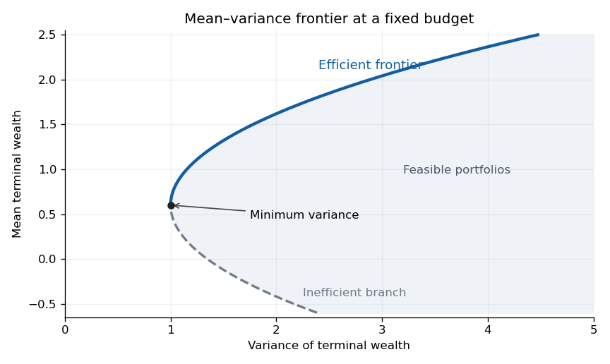

If , then , and only is feasible. The variance minimizer is , still in the stated span; no two-dimensional frontier exists. This degeneracy is not excluded merely by nonsingularity of .
For exponential utility and Gaussian prices, the moment-generating function givesMaximizing this is equivalent to maximizing subject to . Its strictly concave first-order equation givesThus the same two funds suffice.
For the Gaussian two-fund theorem with general utility, the Gaussian assumption and the exponential growth bounds justify the differentiations and expectations. Gaussian integration by parts applied to givesAt any finite maximizer the left side is a multiplier . If is concave and non-affine, and , then is a nondegenerate Gaussian with positive density everywhere. Since continuous is strictly negative on some interval, its expectation is strictly negative. Rearranging provesThe zero portfolio already belongs to that span.
There is a genuine qualification in the final printed assertion: increasing and concave does not exclude affine utility. For , , and , every budget-feasible portfolio is optimal. With , is optimal but is outside the common line spanned by . If is not proportional to , affine utility has no maximizer at all, because a zero-cost direction with positive mean can be scaled without bound. Thus the universal claim about the maximizing portfolio needs non-affine utility and existence of a finite maximizer. Under the literal weaker assumptions there is still a two-fund optimum whenever an optimum exists: the affine constant-mean case permits choosing the minimum-variance portfolio.
For the disc, put . The polar Laplace equation separates aswhere periodicity requires an integer . The radial ansatz gives ; for the solutions are a constant and . Regularity at the origin excludes negative powers and the logarithm.
Writing the boundary data as a Fourier serieswith , , and the analogous formula for , givesEquivalently it is the Poisson integral on the unit disk with kernelFor continuous boundary data this integral converges to the prescribed value at every boundary point, is smooth and harmonic inside, and uniqueness follows from the maximum principle for harmonic functions.
For the square, superpose four solutions, each carrying one side's data and zero data on the other three sides. Set andSeparation of variables gives the explicit sumEach summand has zero Laplacian and the required zero values on three open sides. The Fourier sine series supplies the fourth side. For regular continuous data with matching values at the corners, the harmonic extension also takes the common corner values; termwise boundary evaluation of the sine series at the corners is not valid in general. For incompatible corner data there is no continuous solution on the closed square, but the displayed harmonic solution still attains the prescribed data on each open side.
Suppose first that the unique interior minimum is nondegenerate, , and . Outside a small neighbourhood of the phase exceeds by a fixed positive amount, so that region is exponentially smaller. Inside, expandThe rescaling and a dominated local Gaussian calculation give the Laplace methodIf the minimum is at and , the scale is , giving . At with , replace the denominator by . A stationary quadratic endpoint gives half the interior Gaussian factor.
The printed assumptions do not guarantee nondegeneracy or . More generally, if with and even at an interior minimum, the leading phase scale is and, for , the factor isAt a one-sided endpoint the factor two is absent and the first positive one-sided phase power need not be even. If the amplitude vanishes, expand it to its first contributing term; parity can cancel interior terms. A phase flat to all orders requires its actual local behavior rather than a nonexistent quadratic Taylor coefficient.
The unique minimum is at zero with phase and amplitude . The interior Laplace method givesFor an additional check, extending to the real line gives the exact Gaussian Fourier integral . The omitted tails are exponentially small, so the displayed leading term follows directly.
This is endpoint asymptotics after odd Gaussian cancellation. All interior algebraic terms cancel because is odd. Split the interval into and the remaining tail:The right-hand integral has its minimum phase at its left endpoint, with and nonzero amplitude . Endpoint Laplace method therefore giveThe answer is exponentially small, rather than zero; applying only the interior Gaussian approximation misses the asymmetric boundary tail.
Articles were limited to the first 100 out of 134 total.
Articles by others on the same topic
There are currently no matching articles.