Past exam of the mathematics course of the University of Cambridge / 2010 / ii

For congruence classes in $\mathbb{Z}/N\mathbb{Z}$, defineThese operations are independent of representatives. If $a^{\prime }=a+Nr$ and $b^{\prime }=b+Ns$, then $(a^{\prime }+b^{\prime })-(a+b)=N(r+s)$ and $a^{\prime }{b}^{\prime }-ab=N(rb+sa+Nrs)$. Thus changing representatives leaves both results in the same congruence class. The usual integer laws descend to make this a commutative ring with zero $[0]$ and identity $[1]$.

The decimal expansion gives $M={\sum }_{i=0}^s{a}_{i}10^i$. In modular arithmetic, $10\equiv -1(\mathrm{mod}11)$, and henceAn integer is divisible by eleven exactly when its congruence class is zero, proving both directions of the alternating-digit test.

The Baire category theorem says that a countable intersection of open dense sets in a nonempty complete metric space is dense. Write $E=\{e_1,e_2,\dots \}$. Each singleton is closed in a metric space and has empty interior because there are no isolated points. Therefore every $X\setminus \{e_j\}$ is open and dense. Applying the theorem also to $G$ yieldswhich is dense in $X$. Thus every nonempty open subset meets the required difference, not merely the original dense set $G$.

No. Take the complete metric space $X=\mathbb{R}$ with its usual metric, $E=\mathbb{Q}$, and $G=\mathbb{Q}\cup (1,2)$. This $G$ is uncountable and dense, whereasmisses, for example, the nonempty open interval $(3,4)$. Uncountability does not replace the open-dense hypothesis in the Baire category theorem.

A plane plane crystallographic group is a discrete subgroup of the Euclidean isometry group with compact quotient. Its translations form a normal rank-two Euclidean lattice $\Lambda$; this is the standard translation-lattice structure of a plane crystallographic group. Its point group is the finite group of linear parts, equivalently the quotient by those translations. Conjugating a translation by an isometry sends its translation vector to its image under the linear part, so every point-group element preserves $\Lambda$.

Choose a Euclidean lattice basis. A rotational linear part is then represented by an integer matrix $A$, since it sends the basis to Euclidean lattice vectors. In an orthonormal basis the same map has eigenvalues $e^{i\theta },e^{-i\theta }$, and its trace is independent of basis. ThusThese possibilities give rotation angles, modulo a full turn, $\pi$, $\pm 2\pi /3$, $\pm \pi /2$, $\pm \pi /3$, and $0$, respectively. Consequently the crystallographic restriction theorem isThe restriction comes from integrality of the Euclidean lattice action, not simply from finiteness of the point group.

A binary uniquely decodable code assigns a finite binary word to each source symbol, so that no two distinct finite sequences of source symbols have the same concatenated encoding. This does not require the stronger prefix property. All codeword lengths are positive.

Put $S={\sum }_j{2}^{-l_j}$ and let $A_{k,L}$ count sequences of $k$ source symbols whose encoded total length is $L$. Expanding the product givesUnique decodability makes these encodings distinct, so $A_{k,L}\le 2^L$, the number of binary strings of that length. There are at most $k(l_{\max }-l_{\min })+1$ possible lengths. ThereforeTaking $k$th roots and letting $k\to \infty$ proves the McMillan inequality:

Independence in the Bernoulli logistic-regression model gives the log-likelihoodWriting ${\mu }_i=(1+e^{-\beta x_i}{)}^{-1}$, the score function and curvature areThus a finite maximum-likelihood estimate solves ${\sum }_i{x}_i(y_i-{\hat{\mu }}_i)=0$. If at least one $x_i\ne 0$, the curvature is strictly negative for finite $\beta$, so any such solution is the unique maximizer.

Use the Newton method, which here coincides with Fisher scoring because the second derivative does not depend on the observed responses:Step damping or a bracket for the monotone score provides reliable numerical convergence. If all covariates are zero the parameter is unidentifiable; if the outcomes are separated in the direction of the covariates, the likelihood supremum may occur at $\beta =+\infty$ or $-\infty$ rather than at a finite estimate.

The positive steady state satisfies $1+b(N^{\ast }{)}^2=r$, soWith $N_t=N^{\ast }+{\eta }_t$, the linearization isIts characteristic polynomial is ${\lambda }^2-\lambda +d$, where $d=2(r-1)/r$. The roots are inside the unit disk precisely when $0<d<1$: when they are real they are positive with sum one, and when complex conjugate their common modulus is $\sqrt{d}$. Therefore the fixed point is linearly asymptotically stable for $1<r<2$ and unstable for $r>2$. At $r=2$,This proves period six for the neutral linearized oscillations. The stronger printed claim of a nonlinear period-six branch is not valid for the stated recurrence. It is important to distinguish these two assertions.

Here is a local obstruction, which also checks that the qualification is not merely absence of a proof. Normalize by the moving fixed point, let $x=N_{t-1}/N^{\ast }(r)-1$, $y=N_t/N^{\ast }(r)-1$, and definePut $v=(x,y{)}^T$, $\delta =r-2$, and $Q=x^2-xy+y^2>0$ for $v\ne 0$. The quadratic and cubic terms of $F_2$'s second component are $x^2/2-xy+x^{2}y/2$. Composing six times givesIn particular the quadratic terms cancel, while the cubic components are $-(x+2y)Q/2$ and $(2x-3y)Q/2$. If a small nonzero $v$ were a period-six point, invertibility of $B$ and the norm of this equation would imply $|\delta |=O(|v{|}^2)$. Taking its determinant with $Bv$ then givesSince $Q\ge |v{|}^2/2$, this is impossible for sufficiently small nonzero $v$. Thus no nontrivial nonlinear six-cycle bifurcates locally at $r=2$. At the threshold the same expansion gives $Q(F_2^6(v))=Q(v)-2Q(v{)}^2+O(|v{|}^5)$, so the fixed point is actually locally asymptotically stable nonlinearly, with slow decay. The valid intended linear-stability conclusion is the period-six neutral oscillation above; a literal nonlinear assertion requires a changed model or wording. This is an example of the distinction between linear resonance and nonlinear periodic bifurcation.

The nullclines are $y=\mu x$ and $y=x^2/[\nu (1+x^2)]$. At a nonzero fixed point, cancellation of $x$ yields $\mu \nu =x/(1+x^2)$. The latter function attains its maximum $1/2$ at $x=1$. HenceFor $0<\mu <{\mu }_c$, $x_{-}<1<x_{+}$ and $x_{-}{x}_{+}=1$.

The Jacobian matrix isAt $O$ the distinct eigenvalues are $-\mu ,-\nu$, so the origin is a stable node. At a nonzero fixed point its trace is $-(\mu +\nu )<0$ andThe discriminant is $(\mu -\nu {)}^2+8x/(1+x^2{)}^2>0$. Thus $P_{-}$ is a saddle and $P_{+}$ is a stable node, never a focus.

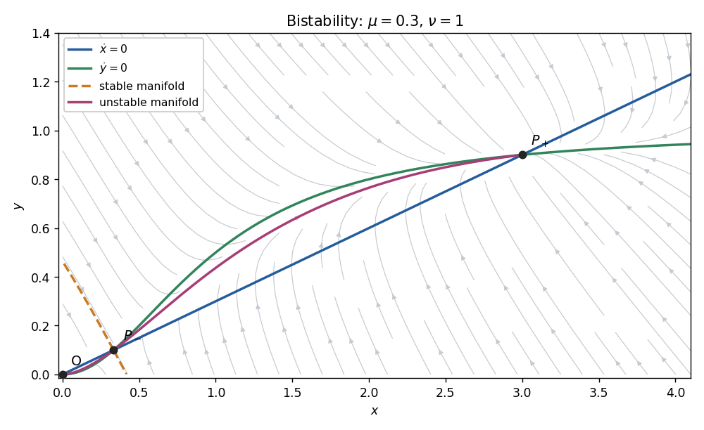
Above the straight nullcline $\dot{x}>0$; below it $\dot{x}<0$. Below the curved nullcline $\dot{y}>0$; above it $\dot{y}<0$. At the saddle, an eigenvector can be chosen as $(1,\mu +\lambda )$: the stable eigenvalue gives negative slope, and the unstable eigenvalue gives positive slope. The stable manifold is the basin boundary. The two branches of the unstable manifold lead respectively to the origin and the positive stable node, as illustrated for representative parameters.

The nonnegative quadrant is forward invariant. Since $\dot{y}\le 1-\nu y$, $y$ stays bounded, and then $\dot{x}=-\mu x+y$ also bounds $x$. Moreover the divergence is the negative constant $-(\mu +\nu )$, excluding periodic or homoclinic loops by the Bendixson-Dulac criterion. The Poincaré-Bendixson theorem then leaves convergence to a fixed point. Initial data on the saddle's stable manifold approach the saddle; data in the two open basins approach extinction at $O$ or persistence at $P_{+}$, respectively.

The real part of a holomorphic function is real analytic and has a local complexification in its two real coordinates. Define $f^{\ast }(w)=\overline{f(\bar{w})}$. On real $(x,y)$,and the same identity holds after analytic continuation to complex $(x,y)$. Substituting $x=(z+{\bar{z}}_0)/2$ and $y=(z-{\bar{z}}_0)/(2i)$ gives $x+iy=z$ and $x-iy={\bar{z}}_0$, henceThe conjugation on the final constant is present in the PDF but was lost in the converted TeX. Without it the formula already fails when $z=z_0$ and $f(z_0)$ is not real.

Now $z{e}^{iz}=(x+iy)e^{-y}(\cos x+i\sin x)$ has the specified real part. Thus the complete family isAny two such holomorphic functions differ by a holomorphic function with zero real part; the Cauchy-Riemann equations make its imaginary part constant on a connected neighborhood.

In Lagrangian mechanics, the energy balance for an autonomous Lagrangian uses $E={\sum }_i{\dot{q}}_i\partial L/\partial {\dot{q}}_i-L$. For the stationary vector potential the velocity-linear magnetic term cancels in this expression, leaving kinetic energy. In cylindrical coordinates,Time independence and the cyclic angular coordinate give two constants:The three Euler-Lagrange equations areThe supplied angular velocity is $\dot{\varphi }=-2eg(z_0)/m$. Set $r=r_0$, $z=z_0$ and use this constant angular velocity. The radial right-hand side is $m{r}_0({\dot{\varphi }}^2+2eg\dot{\varphi }/m)=0$, the angular momentum is constant, and the vertical equation vanishes when $g^{\prime }(z_0)=0$. These equations and the initial data therefore giveFor nonzero radius and charge this is the requested circular orbit.

The Hubble time is the instantaneous inverse expansion rate $H_0^{-1}$, where $H=\dot{a}/a$. A radial light ray covers comoving distance $\int cdt/a(t)$. Since $a(t_0)=1$, the present proper radius of the particle horizon isFor the power-law scale factor, $a(0)=0$ requires $\alpha >0$. The integral converges only when $\alpha <1$, in which caseAt $\alpha =1$ the divergence is logarithmic, and at $\alpha >1$ it is a power divergence. The familiar flat-universe epochs have $\alpha =1/2$ for radiation and $\alpha =2/3$ for pressureless matter, obtained from $\rho \propto a^{-4}$ or $a^{-3}$ and the Friedmann equation. Both have $0<\alpha <1$, so their ages are less than the present Hubble time. These power laws describe idealized single-component epochs rather than the full late-time expansion history.