Past exam of the mathematics course of the University of Oxford / 2015 / Prelims / Mathematics V resit (A10142W1)

Source: released examination PDF, bundle pages 234–237.

Here $\varphi$ is a scalar field: the source's description as a vector field is a typographical slip, since the displayed formula is for its gradient. For cylindrical coordinates, write $x=r\cos \theta$, $y=r\sin \theta$. Away from $r=0$, a local choice of $\theta$ gives the partial derivativesThe chain rule therefore givesUse the Cartesian coordinates definition $\nabla \varphi ={\varphi }_x{\mathbf{e}}_x+{\varphi }_y{\mathbf{e}}_y+{\varphi }_z{\mathbf{e}}_z$ and the unit vectorsCollecting their coefficients provesThis is the gradient in cylindrical coordinates. The factor $1/r$ converts a change in angle into a change per unit arc length.

In cylindrical coordinates, $(-y,x,0)=r{\mathbf{e}}_{\theta }$ and $x+r=r(1+\cos \theta )$. Hence the vector field simplifies toTake the orientation of $C$ to be increasing $\theta$, as in its given parametrization. On the circle, $d\mathbf{r}=a{\mathbf{e}}_{\theta }d\theta$, so its line integral isWe used $\sqrt{1+\cos \theta }=\sqrt{2}|\cos (\theta /2)|$; the cosine is nonnegative on this interval. In particular, the answer does not depend on $a$.

Here a potential of a conservative vector field means a single-valued scalar field $\psi$ with $\nabla \psi =\mathbf{F}$. By the fundamental theorem for line integrals, its line integral around every closed curve must vanish. Here the angular circulation obstruction to a cylindrical potential lets us test this using a circle about the axis.

On $V_1$, the circle from i lies entirely in the region and has line integral $4\sqrt{2}$. Therefore there is no potential of a conservative vector field on $V_1$.

On $V_2$, choose the continuous angular branch $-\pi <\theta <\pi$. By a, the equation for a potential of a conservative vector field reduces to ${\psi }_r={\psi }_z=0$ and ${\psi }_{\theta }=\sqrt{2}\cos (\theta /2)$. ThusThe denominator is positive throughout $V_2$, including when $y=0$ and $x>0$, so this is a well-defined differentiable potential of a conservative vector field on the entire region.

For $V_3$, choose the particular circle $x=2\cos \theta$, $y=2\sin \theta$, $z=0$. Its only point on the removed half-plane's supporting cut is $(-2,0,0)$, where $(x+2{)}^2+z^2=0<1$; this point is retained by $V_3$. Thus the whole circle lies in $V_3$ and again has line integral $4\sqrt{2}$. Consequently there is no potential of a conservative vector field on $V_3$. The opening in the cut allows a closed curve to go around the excluded axis.

Finally $V_4\subset V_2$. Restricting the potential of a conservative vector field already constructed on $V_2$ givesThe extra excluded cylinder does not invalidate an existing potential of a conservative vector field. Thus being simply connected is a sufficient condition in the usual curl-free criterion, not a necessary condition for a particular vector field to have a potential of a conservative vector field.

For a bounded region $V\subset {\mathbb{R}}^3$ with piecewise smooth boundary, suppose $\mathbf{F}$ is a continuously differentiable vector field on an open neighbourhood of its closure. The divergence theorem, with outward unit normal vector $\mathbf{n}$, isThe surface integral measures total outward flux. Edges and isolated vertices have zero surface area and do not affect the integral.

In Cartesian coordinates, write the constant vector as $\mathbf{c}=(c_1,c_2,c_3)$. The product rule and constancy of its components giveThe last expression is the dot product with the gradient, so

Apply the divergence theorem to $\varphi \mathbf{c}$, using ii. Because the vector $\mathbf{c}$ is constant, it can be taken outside both integrals:This holds for every $\mathbf{c}$, in particular each of the three Cartesian basis vectors. Equality of the three components proves the gradient volume-to-boundary identityIt suffices that $\varphi$ be a continuously differentiable function on a neighbourhood of the closure of $V$.

Use cylindrical coordinates. The real square root restricts the projection to $0\le r\le 1$, and there $r-1\le 0\le \sqrt{1-r^2}$. Since $\nabla x={\mathbf{e}}_x$, the volume integral isFor an independent boundary calculation, split $\partial V$ into an upper hemisphere $S_{+}$ and a lower right circular conical surface $S_{-}$. They meet in the circle $r=1,z=0$ and there is no additional planar face.

On $S_{+}$, use the parametrizationThe outward unit normal vector is $\mathbf{R}$, and the surface area element is $\sin \alpha d\alpha d\theta$. The $y$ and $z$ components of ${\iint }_{S_{+}}x\mathbf{n}dS$ vanish by the angular integrals of $\sin \theta \cos \theta$ and $\cos \theta$. The $x$ component isOn $S_{-}$, the parametrization $(r\cos \theta ,r\sin \theta ,r-1)$ has outward vector area elementIts negative vertical component points out below the solid. Multiplying by $x=r\cos \theta$ and using the same angular symmetry in integration givesTherefore the independently evaluated surface integral isin agreement with the volume integral. The isolated apex of the cone does not contribute to the surface integral.

The annulus is $1\le r\le 2$ in polar coordinates. Their Jacobian determinant supplies $dxdy=rdrd\theta$, so

The original double integral covers the triangle $0\le y\le x\le 1$. By Fubini's theorem, after reversing the order, $y$ runs from $0$ to $1$ and $x$ from $y$ to $1$. Since a continuous function is integrable on this bounded region,For the square pyramid, a horizontal section at height $z$ is a square of side $2(1-z)$: each vertex moves linearly from the base towards $(1,1,1)$. Hence its cross-sectional area is $4(1-z{)}^2$, and its volume is $4{\int }_0^1(1-z{)}^{2}dz$. To use the identity just proved, choose $f(y)=1-y$:

Start with the solid between the elliptic paraboloid $z=x^2+y^2$ and the upper plane $z=10-2y$. Its projection is the disksince their vertical separation is $11-x^2-(y+1{)}^2$. The second lower bound, $z\ge 2-2x$, removes the part between the elliptic paraboloid and this lower plane whereverCall this second disk $E$. Its centre is distance $\sqrt{2}$ from the centre of $D$, andbecause $5+2\sqrt{6}<11$. Thus $E$ lies wholly inside $D$. In particular the lower plane never exceeds the upper plane on $E$, so the subtraction describes exactly the requested solid.

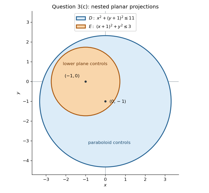
The nested-disk subtraction for paraboloid volumes therefore gives a difference of two double integrals:Translate polar coordinates to the centre of each disk. A general integral of this form isUsing $A=11$ and $A=3$ gives

Assume the rod has constant cross-sectional area $A$, no internal source of heat, no bulk motion, and no lateral heat flux. Assume also that each section has a uniform temperature, so that $T$ depends only on $x,t$, and that Fourier's law applies with the stated constant thermal conductivity $k$. The longitudinal heat flux density is then $q=-k{T}_x$.

By conservation of energy, the rate of increase of internal energy in a slice $[x,x+\Delta x]$ equals incoming minus outgoing heat:Divide by $A\Delta x$ and take the limit $\Delta x\to 0$. For a sufficiently differentiable temperature field this gives $\rho c{T}_t=-q_x=k{T}_{xx}$, and henceHere $\rho$ is mass density, $c$ is specific heat capacity, and $\kappa$ is thermal diffusivity.

A steady state has $T_s^{\prime \prime }=0$, so $T_s=a+bx$. The fixed temperature gives $T_s(0)=T_0$, and thermal insulation gives $T_s^{\prime }(L)=0$. ThusSubtracting this steady state produces the homogeneous mixed boundary conditionsThe partial differential equation and boundary conditions apply for $t>0$. The initial condition is attained as $t\downarrow 0$. Its slope at $x=L$ is $-T_0/L$, so it does not satisfy the insulated-end condition at the instant $t=0$. The resulting heat equation solution is smooth for $t>0$ and approaches the initial temperature continuously; its spatial derivative need not be continuous at $(L,0)$.

For separation of variables, put $U=X(x)H(t)$ and set $X^{\prime \prime }/X=H^{\prime }/(\kappa H)=-\lambda$. The boundary conditions are $X(0)=0$, $X^{\prime }(L)=0$. Multiplying $-X^{\prime \prime }=\lambda X$ by $X$ and using integration by parts givesA nonzero solution therefore has $\lambda >0$: the zero case forces $X$ constant, and then $X(0)=0$ forces $X=0$. Writing $\lambda ={\mu }^2$, the eigenfunctions and their temporal factors areThese sine functions are orthogonal on $[0,L]$, with squared norm $L/2$. Expanding the initial condition and multiplying by $\sin ({\mu }_{m}x)$ gives, using the permitted interchange of the sum and integral,Here $\cos ({\mu }_{n}L)=0$ and $\sin ({\mu }_{n}L)=(-1{)}^n$. Thus the Fourier series solution isThe exponential decay permits differentiation of the series for $t>0$, and each term satisfies both boundary conditions. At $t=0$ it is the mixed-end Fourier expansion of $-T_{0}x/L$.

The gained heat is the increase in internal energy. Since the paper specifies no cross-sectional area, first give the answer per unit cross-sectional area; multiply by $A$ for a rod of cross-sectional area $A$. The initial temperature has integral $T_{0}L/2$, whereas ${\int }_0^L\sin ({\mu }_{n}x)dx=1/{\mu }_n$. At $t_{\ast }=L^2/\kappa$ this givesNumerically $\Delta Q/A\simeq 0.45623855\rho c{T}_{0}L$. This is positive and less than the eventual gain $\rho c{T}_{0}L/2$, as expected from relaxation towards the uniform steady state.

Assume $\rho$ is mass per unit equilibrium length, the tension has constant magnitude $T$, the string has negligible bending stiffness, and there is no damping or external transverse force. Assume small slopes $|y_x|\ll 1$ and purely transverse motion. Then a short segment has mass $\rho \Delta x$ to first order. If $\alpha$ is the angle of its tangent, the small-slope approximation gives $\sin \alpha \simeq \tan \alpha =y_x$.

The vertical components of tension at the two ends give net transverse force $T[y_x(x+\Delta x,t)-y_x(x,t)]$. Newton's second law therefore givesto first order. Dividing by $\Delta x$ and taking its limit to zero yieldsThus $c$ is the propagation speed of small transverse waves.

Write $y(x,t)=Y(\xi ,\eta )$ with $\xi =x-ct$, $\eta =x+ct$. The chain rule gives the differential operatorsTheir squared difference isConsequently the wave equation becomes $Y_{\xi \eta }=0$. Integrating first in $\eta$ gives $Y_{\xi }=F^{\prime }(\xi )$; integrating in $\xi$ gives the general solutionThe arbitrary twice differentiable functions describe right-moving and left-moving waves, respectively. Conversely the chain rule shows that each such sum satisfies the wave equation.

Enforce the fixed-end Dirichlet boundary condition by taking the odd extension of the initial velocity to the whole line:This agrees with the specified initial condition for $s\ge 0$. To derive the relevant form of D'Alembert's formula, the zero initial displacement in b gives $G=-F$, up to a cancelling constant. The initial velocity then gives $-2c{F}^{\prime }=v_o$. HenceAn antiderivative, valid across $s=0$, isEvaluation therefore gives the solution throughout $x>0,t>0$:For $ct\le x$, replace $|x-ct|$ by $x-ct$; for $ct\ge x$, replace it by $ct-x$. Thus the same expression includes the reflected wave after it reaches the fixed end.

At $x=0$ the two terms agree, so $y(0,t)=0$. At $t=0$ they again agree, so $y(x,0)=0$. Differentiating the integral with respect to $t$ giveswhich recovers $y_t(x,0)=\kappa x{e}^{-x/L}$. Since $v_o$ is a continuously differentiable function, the formula is twice continuously differentiable even across $x=ct$, and satisfies the wave equation there as well.

Let $w$ be the difference of two solutions. It is a harmonic function in the open rectangle, continuous on its closure, withInterpret these Neumann boundary conditions classically on the open edges, with the corresponding first derivatives extending there. We use the strong maximum principle for harmonic functions together with even reflection across a homogeneous Neumann boundary. This avoids imposing differentiability at the two bottom corners, where the original data fail a corner compatibility condition for mixed boundary data.

By continuity on the compact rectangle, $w$ attains a maximum $M$. Suppose $M>0$. It cannot occur on the bottom edge, where $w=0$. If it occurs in the interior, the strong maximum principle for harmonic functions makes $w$ constant, contradicting its bottom value. If it occurs on an open vertical or top edge, the zero normal derivative allows an even reflection across that edge. The reflected harmonic function then has an interior maximum, giving the same contradiction.

The only remaining possibilities are the two top corners. Reflect evenly across both meeting edges. This gives a bounded harmonic function on a punctured neighbourhood of the corner. The removable singularity for a bounded harmonic function fills the centre with its continuous value. The corner is now an interior maximum, again impossible. Therefore $w\le 0$. Applying the identical argument to $-w$ gives $w\ge 0$.

Thus $\boxed{w=0}$, and the solution is unique among the continuous classical solutions with the stated edge conditions.

For $0<y<\pi$, define $J(y)={\int }_0^{\pi }{u}_y(x,y)dx$. Differentiate under the integral and use Laplace's equation:Thus $J$ is constant. The top Neumann boundary condition gives $J(\pi )=0$, soFor the included endpoint $y^{\ast }=0$, the integral is interpreted as an improper integral at the bottom corners if necessary. The Fourier series constructed in c gives, on $0<x<\pi$,The second series is absolutely and uniformly convergent; the first term has only integrable logarithmic singularities. Its integral is zero since ${\int }_0^{\pi }\log (2\sin x)dx=0$, while every cosine term also has zero integral. This proves the endpoint as well:For completeness, the logarithmic integral follows without any endpoint differentiation. Put $I={\int }_0^{\pi /2}\log (\sin x)dx$ and substitute $x\mapsto \pi /2-x$ to obtain $I={\int }_0^{\pi /2}\log (\cos x)dx$. Adding and using $\sin x\cos x=\sin (2x)/2$ gives $2I=I-(\pi /2)\log 2$, hence $I=-(\pi /2)\log 2$ and the required full-interval result.

For separation of variables, set $u=X(x)Y(y)$, with $X^{\prime \prime }/X=-Y^{\prime \prime }/Y=-\lambda$. The side Neumann boundary conditions give $X^{\prime }(0)=X^{\prime }(\pi )=0$. As in the standard Sturm-Liouville problem, integration by parts shows $\lambda \ge 0$. The zero eigenvalue gives constant $X$, and $Y^{\prime \prime }=0$ together with $Y^{\prime }(\pi )=0$ makes $Y$ constant too.

For positive eigenvalues, the side conditions give $\lambda =n^2$, $X_n=\cos (nx)$, $n\ge 1$. The top condition chooses the hyperbolic cosine factor $\cosh (n(\pi -y))$. Normalize it to one at $y=0$, obtainingThe orthogonality of integer Fourier modes and the permitted interchange of summation and integration giveFor the remaining Fourier coefficients, integrate by parts twice. The sine boundary term vanishes, and with $f=x(\pi -x)$,The last integral vanishes because $f^{\prime \prime }=-2$ and $n$ is a positive integer. Thus $a_n=-2(1+(-1{)}^n)/n^2$: only even Fourier modes survive, as expected from reflection symmetry about $x=\pi /2$. Writing $n=2m$ givesThe factor involving hyperbolic cosine lies between zero and one on the closed rectangle. Comparison with $\sum m^{-2}$ proves uniform convergence, so the solution is continuous on the entire boundary and takes the prescribed bottom values. On every strip $y\ge \epsilon >0$, the Fourier coefficients have additional exponential decay, allowing differentiation and verifying Laplace's equation and all three Neumann boundary conditions.

To justify the endpoint calculation in b, differentiate at $0<x<\pi$, $y=0$ in the interior-edge sense:Subtracting $1$ from the hyperbolic tangent leaves an absolutely convergent series. For the remaining part, the power series $-\log (1-z)={\sum }_{m\ge 1}{z}^m/m$ gives, by taking real parts at $z=r{e}^{2ix}$ and then $r\uparrow 1$,The same formula follows as the limit of the differentiated interior solution, since its leading multiplier is $e^{-2my}$. This establishes the boundary normal derivative used in b. It also explains why the failure of the corner compatibility condition for mixed boundary data affects first derivatives at the bottom corners without spoiling continuity of $u$ itself.

Use the convention that the Newtonian gravitational potential tends to zero at infinity and the gravitational field is $-\nabla \varphi$. A source element of mass $dm$ at position vector ${\mathbf{r}}^{\prime }$ contributes $-Gdm/|\mathbf{r}-{\mathbf{r}}^{\prime }|$, where $G$ is the gravitational constant. For the curve, $dm=\gamma d{s}^{\prime }$, soHere $d{s}^{\prime }$ is arc length along the source curve; the expression is finite away from it. This normalization fixes the otherwise arbitrary additive constant.

For the surface, a source element has mass $dm=\sigma d{S}^{\prime }$. Superposing its Newtonian gravitational potential gives the surface integralHere $d{S}^{\prime }$ is the source surface area element, ${\mathbf{r}}^{\prime }$ the source position vector, and $G$ the gravitational constant. The same zero-at-infinity convention applies.

For a volume source of constant mass density $\rho$, use $dm=\rho d{V}^{\prime }$. Its Newtonian gravitational potential is the volume integralThe source and observation position vectors are ${\mathbf{r}}^{\prime }$ and $\mathbf{r}$, respectively; $G$ is the gravitational constant. With this sign convention positive source mass gives negative Newtonian gravitational potential.

Write the observation point as $(0,0,h)$ with $h>0$, reserving source coordinates for the integral. For the straight segment, $d{s}^{\prime }=d{x}^{\prime }$ and the separation is $\sqrt{x^{\prime 2}+h^2}$. Therefore its Newtonian gravitational potential isEquivalently $\varphi (h)=-2G\gamma \mathrm{arsinh}(a/h)$. At large $h$ it approaches $-G(2a\gamma )/h$, the Newtonian potential of a point mass with the segment's total mass.

Use source polar coordinates $x^{\prime }=s\cos \theta$, $y^{\prime }=s\sin \theta$ on the semicircular disk, with $0\le s\le a$ and $0\le \theta \le \pi$. Its surface area element is $sdsd\theta$, and the separation from $(0,0,h)$ is $\sqrt{s^2+h^2}$. ThusThis Newtonian gravitational potential is half that of the full disk because the separation is independent of the polar angle. At large $h$ it approaches $-G(\pi a^2\sigma /2)/h$, with the correct total mass.

Use source spherical coordinates with radius $s$, polar angle $\alpha$ measured from the positive $z$-axis, and azimuth $\theta$. The lower half of the spherical shell has $a\le s\le 2a$, $\pi /2\le \alpha \le \pi$, and $0\le \theta \le 2\pi$. Its volume element is $s^2\sin \alpha dsd\alpha d\theta$. At the observation point $(0,0,h)$, $h>0$, the separation is $\sqrt{s^2+h^2-2sh\cos \alpha }$, soThe angular integral is elementary: put $q=\cos \alpha$ to obtainWe used $\sqrt{(s+h{)}^2}=s+h$ since both $s,h$ are positive. HenceThus the axial potential of a uniform hemispherical shell, at every point of the positive $z$-axis, isThere is no need to split into $h<a$, $a<h<2a$, and $h>2a$: the observation point is outside the lower hemisphere in all three cases. As checks, $\varphi (h)\to -3\pi G\rho a^2$ as $h\downarrow 0$, and at large $h$,The last factor is exactly the total mass of the lower half of the spherical shell.