The numerator is the derivative of the denominator. Using the chain rule in reverse gives the antiderivativeThe absolute value makes this real on every interval where the denominator is nonzero. The integration constant may be chosen independently on the intervals separated by .
The quotient rule simplifies the derivative toIts zeros are and , both in the domain. Substitution gives the two stationary pointsThe first is a local maximum and the second a local minimum, since the numerator of changes sign from positive to negative at and from negative to positive at . The denominator of the original rational function vanishes atThe numerator is nonzero at both values, so these discontinuities are poles, not removable holes.
Direct matrix multiplication givesSubtracting verifies . This is also the Cayley-Hamilton theorem for the characteristic polynomial .
For , the first two derivatives at one are and . The Taylor expansion beginsAll three displayed terms are nonzero terms of the expansion about one.
This is a separable differential equation. Multiply by and integrate:The initial condition gives . HenceFor a real solution the outer logarithm requires a positive argument. The maximal interval containing the initial point is therefore . At either endpoint diverges, so the real solution cannot continue through it with a finite value.
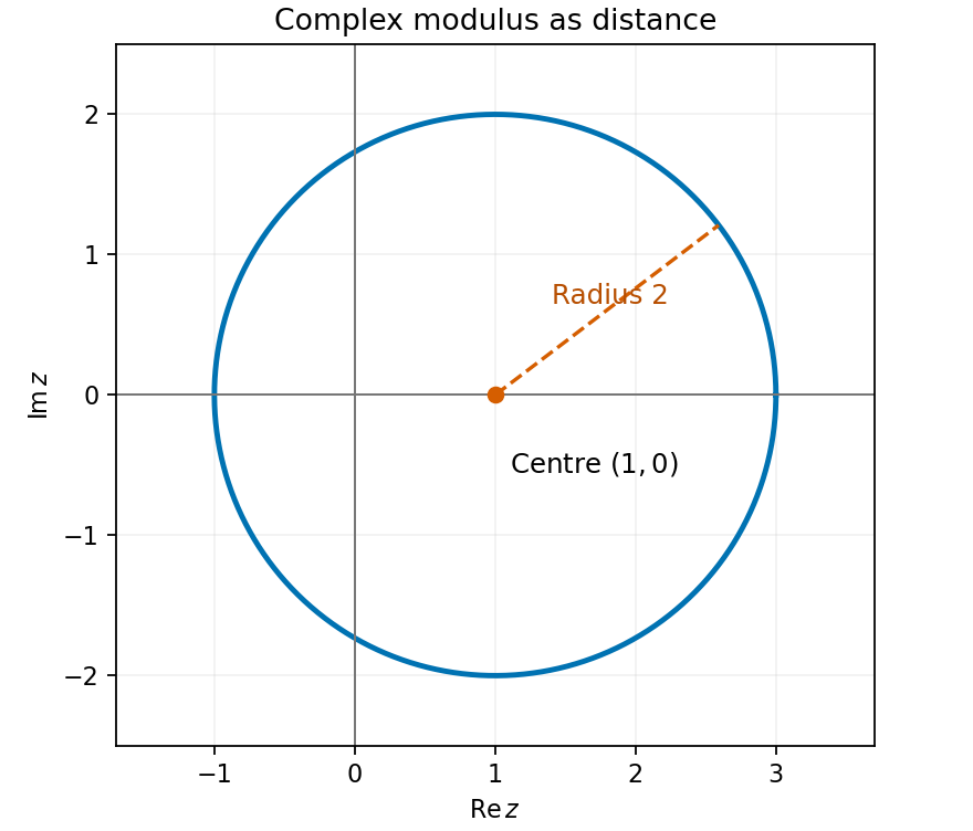
Write . The complex modulus condition is equivalent to . Thus the locus is a circle of radius two centred at in the complex plane. Its extreme points are , , and .
The derivative is , giving slope twelve at . The point on the curve is . The point-slope equation of the tangent line is consequently
In Cartesian coordinates, the divergence uses the matching coordinate for each component:Each of these three partial derivatives vanishes.
The gradient part contributes zero around a closed path by the fundamental theorem for line integrals:Along the parametrization, , so the first two components of vanish wherever the printed expression is defined. The remaining component gives . ThusThe printed field needs a qualification: is undefined at the isolated parameters where , so cannot literally be evaluated. The result above is the improper line integral, or equivalently the integral of the continuous extension of the restricted field along the curve. That restricted field tends to at each omitted parameter. No extension of the full field to a neighbourhood is being assumed.
The curl of a gradient vanishes because the mixed second partial derivatives of the smooth function agree. Therefore everywhere, andUnlike part (i), this integrand does not involve the problematic auxiliary field.
Where is twice continuously differentiable, the identity divergence of a curl is zero gives . All regular portions of the parameter interval lie in this region, henceas an improper line integral. Besides the endpoint problem from (i), the curve touches at , where the printed real expression has no smooth open neighbourhood. The identity applies on the intervening open segments, and its zero value has a unique continuous extension along the curve. A literal classical integrand at every parameter is not supplied by the printed field.
Writing , the gradient is . Its divergence, equivalently the Laplacian of , isOn the unit sphere this scalar is the constant . The lower hemisphere has surface area , soThis is a scalar surface integral of the divergence, not the electric- or vector-field flux integral. There is no normal component to insert.
The scalar integrand still equals throughout the unit sphere, and the upper hemisphere has the same surface area . Excluding its equator changes no area. ThereforeThere is no sign reversal between hemispheres because this scalar surface integral has no choice of normal orientation.
Using the physics convention for spherical coordinates, the polar angle is measured from positive and the azimuth from positive toward positive . The Cartesian coordinates are
Hold fixed and differentiate the position vector . Its coordinate tangent vectors areTheir dot product is zero, and their squared Euclidean norms are and . To first order, the displacement is . Squaring givesThis is the line element on a sphere. The chord distance and the short surface arc length agree to the order retained here.
A plane through the origin has equation for some nonzero normal . Dividing that normal by its Euclidean norm makes without changing the plane. Substitute the spherical coordinates from (a) and cancel the nonzero radius:Its intersection with the sphere is the desired great circle; changing the sign of all three coefficients describes the same circle.
At the first endpoint, the Cartesian coordinates are , so its great circle must have . At the second endpoint, the plane condition gives . Since , an equivalent regular plane equation isWhere , divide by to obtainThe regular implicit equation includes the equatorial first endpoint; the tangent form is undefined there and must be read by a limit. The shorter connecting arc of this great circle is the shortest path. The endpoints are not antipodal, so this shorter arc is unique. For example, the central angle is , giving spherical distance .
For , the exponential definitions of the hyperbolic functions give and . Taking reciprocals of these positive quantities proves . Also for , so division by the positive gives . Combining,
The specified unit vector is ; the positive component selects that direction. The gradient is , giving at the point. The directional derivative is therefore
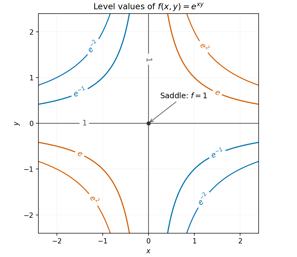
Since , a level can occur only for . Taking its natural logarithm gives . Thus produces rectangular hyperbolas in the first and third quadrants, produces them in the second and fourth quadrants, and consists of both coordinate axes.
The gradient vanishes only at , where . The Hessian matrix there is , with negative determinant. Equivalently, while for nonzero small . Hence the only stationary point is a saddle point at on the graph; its location in the contour plane is the origin.


Expand the determinant along the first row:Thus . The signs in the middle cofactor account for its positive contribution.
The characteristic polynomial, using the convention , isIts zeros give the eigenvalues, including algebraic multiplicity:Their product is and their sum is , agreeing with the determinant and trace of the matrix.
For , the eigenvalue equation reduces to a one-dimensional eigenspace spanned by . For , the rows of are multiples of , so its eigenspace is the plane . One possible set of three independent eigenvectors isEvery eigenvector for is a nonzero linear combination of the last two. Their two-dimensional eigenspace shows that the repeated root is not defective: the matrix is diagonalizable.
For the particular eigenvectors chosen in (iii), the dot products areThus only and are orthogonal for this choice. The matrix is not symmetric, so distinct eigenvalues alone do not imply orthogonality. Another basis within the repeated eigenspace may change which chosen vectors are perpendicular; the dot products above specify the convention completely.
The transpose reverses product order, so . If is an orthogonal matrix, then and the given identity becomesMultiply on the left by to obtain . Therefore is antisymmetric, so it is an antisymmetric matrix, namely .
Take determinants of . In order three, multiplication of a matrix by minus one changes its determinant's sign. HenceThe assumption is the same as , so multiplication by givesSince the matrices are real, the first factor is strictly positive. Thus , proving that is a singular matrix. This is singularity forced by an odd-dimensional transpose-inverse identity; no orthogonality of was used.
First solve for the velocity components. The integrating factor givesIntegrating once more and imposing the initial position givesThese formulas describe projectile motion with linear drag. Differentiation checks both second-order differential equations and both initial velocities. At large positive time, the horizontal velocity tends to zero and the vertical velocity tends to the terminal value .
If , the first formula in (a) gives andSubstitute this and into :For finite physical times , the domain is , valid for either sign of . If , the trajectory is vertical, , and in general no single-valued graph describes it. As a consistency check, the logarithmic expansion at fixed cancels the apparent terms and gives as , the drag-free parabola.
Use the integration by substitution , with . On this interval , so it cancels the positive denominator square root. The transformed integral isIts integrand is even. Therefore the answer in the PDF's modulus-amplitude convention for the elliptic integral of the second kind isThe modulus is , not the squared parameter .
Differentiating the parametrization gives and . Thus the arc length element isAll four quadrants give the same contribution. Consequently the ellipse perimeter isThe final factor is the complete elliptic integral of the second kind, evaluated at the eccentricity of a conic .
For small , the binomial series gives the uniform expansion . Since , integration yieldsAlso , so the familiar symmetric approximation is equivalent to this order. This is the first correction in the ellipse perimeter expansion near a circle; the two approximate formulas need not agree at order .
Temporarily label the individual pieces. A random placement is a uniform injection of thirty-two distinct pieces into sixty-four squares, giving equally likely outcomes. For a colour-matching placement, the black pieces have available injections, and independently the white pieces have the same number within their disjoint set of squares. ThereforeHere . Treating same-colour pieces as indistinguishable gives the same probability, because the common within-colour labeling factors cancel. The two colour choices in the favourable count occupy disjoint square sets; no independence assumption about unrestricted placements is required.
The lazy choice weights are and , in ratio three to one. Normalizing gives . Let denote selection of the first question and let . Its conditional expected value, divided by , isso . If the overall lazy fraction is , the law of total probability gives . Bayes' theorem then givesSolving yields . The observed mean is conditioned on the chosen question, so it cannot be equated directly to the unconditional mean over all students.
The integrand separates into a radial and an angular factor, soThe differential printed in the PDF is already . No further polar Jacobian is to be inserted into this given iterated integral.
The intersections satisfy , or , so the bounded region has . Over that interval the parabola is above the line, and their height difference is . Thus its area isUsing upper minus lower ensures a positive geometric area.
The projection onto the - plane is the disk . In polar coordinates, the height is and the polar area element is . The volume is thereforeThe radial factor here is required because this integral is being constructed from the geometric volume, unlike the already specified integral in (a).
Put . In the right half-plane,The last two cancel, so . The possible singular point lies outside the open domain .
For , a level curve of value has . These are rays from the origin, restricted to the right half-plane. For positive , the values increase with angle from on the lower boundary to on the upper boundary. If , the function is identically zero. The left panel of the figure in (c) shows these ray-shaped level curves.
Let . Direct partial differentiation, away from , givesThese are the Cauchy-Riemann equations. Equivalently, with , the analytic mapping is , the inverse Cayley transform between the half-plane and disk.
The supplied harmonicity result can also be checked by the multivariable chain rule. The Cauchy-Riemann equations imply , , and . HenceThis is conformal invariance of harmonicity for the given mapping.
Simplify the real component to . Thus is the unit circle with excluded from the mapping's domain. Its upper semicircle has and its lower semicircle has ; the point maps to . Inside the disk, , so the principal arctangent is unambiguous. Setting givesThe Laplace equation follows from (b). Approaching an open upper boundary arc makes the ratio tend to , giving ; the lower arc gives . This solution is in terms of the harmonic measure of a semicircle in a disk .
The boundary data jump at , so no path-independent continuous boundary value can be imposed at those two junctions. The displayed bounded harmonic function is the solution with the specified limits on the open arcs; those endpoint discontinuities are part of the idealized capacitor geometry.
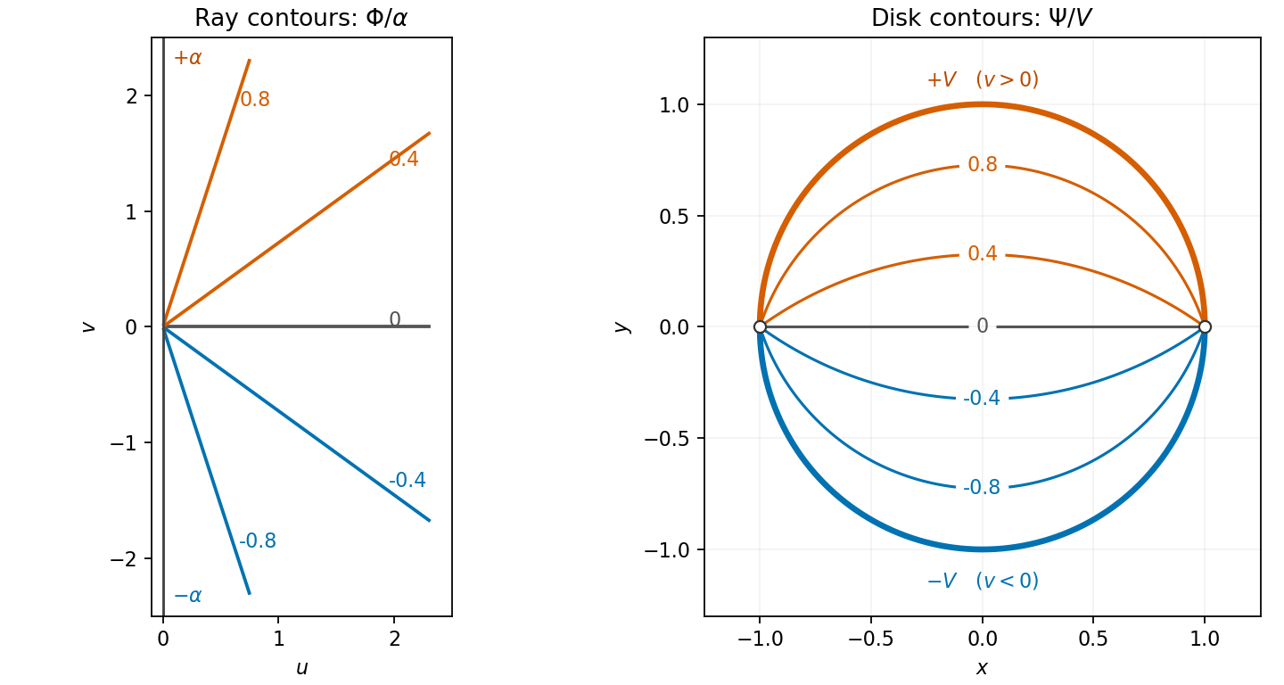
Harmonic ray contours in the right half-plane and the potential in a disk with opposite semicircle boundary values
. Details. 
Apply the Leibniz rule to the th derivative in Rodrigues' formula. If derivatives fall on and on , the corresponding term is . Cancelling the prefactor givesThe leading coefficient is nonzero, so this is a polynomial of degree exactly . In particular, the requested coefficients in areThese are the ordinary Laguerre polynomials, with normalization .
Differentiating gives . Applying the Leibniz rule times to this identity givesOnly two terms survive on each side because the multiplying factors are linear. Rearranging yields . Since , the next two derivatives are and . Substituting and cancelling givesThis is deriving the Laguerre equation from Rodrigues' formula, exhibiting as an eigenfunction of the Laguerre differential operator on polynomials.
Articles were limited to the first 100 out of 102 total.
Articles by others on the same topic
There are currently no matching articles.