Expanding the cross product gives . Comparing its three components in order from the last to the first gives , , and . ThereforeThe nonzero value of permits division to find , and the resulting nonzero determines .
The chain rule identifies an antiderivative directly:The upper limit in the PDF is . By the fundamental theorem of calculus, the required integral is
The determinant is , so the matrix inverse exists. Using the two-by-two adjugate matrix formula givesMultiplication on either side gives the identity matrix, which also checks the signs of the off-diagonal entries.
Multiply by the complex conjugate of the denominator:Thus the real part and imaginary part are respectively
Near , use , so and . The Taylor series therefore beginsThe constant term is one of the requested three terms. The local expression is legitimate because this neighbourhood has .
The partial derivatives are and . Since the exponential function never vanishes, substituting into the partial differential equation gives . Hence
The implication means that , so . By the definition of conditional probability,This implication gives ; it does not make the two events independent.
In Cartesian coordinates, calculate the divergence by differentiating each component with respect to its matching coordinate:For the curl, take the alternating cross-derivatives:
Parametrize the directed segment by , . Its tangent is , while the restricted vector field is . The line integral is thereforeAlternatively, , so the fundamental theorem for line integrals gives the same endpoint difference.
The derivative is . Thus a stationary point occurs either at or where . Since on the specified open interval, the only allowed cosine zeros are and . The five stationary abscissae areTheir ordinates are , , and , respectively. For completeness, shows that the inner pair are local minima and the outer pair are local maxima; is also a local maximum because .
Solving gives and . A convenient normalized eigenvector isThe displayed nonzero vector proves that four is an eigenvalue. Every nonzero multiple represents the same eigendirection.
A vector perpendicular to has the form . Direct matrix multiplication givesThus every nonzero such vector is an eigenvector with . The zero vector must be excluded from the literal claim about “any” perpendicular vector, since an eigenvector is nonzero. The eigenspace is two-dimensional. Equivalently, exhibits the spectrum of a scalar matrix plus a rank-one projector.
Choose two perpendicular unit directions in the eigenspace:Their pairwise dot products vanish and their Euclidean norms are one. They form an orthonormal basis of eigenvectors, with eigenvalues , as guaranteed for a real symmetric matrix by the spectral theorem for real symmetric matrices.
The trace is the sum of the eigenvalues, counting multiplicity, while the determinant is their product:A direct expansion along the middle row checks the latter: .
Using the ordered orthonormal basis chosen in (c), the column matrix isOther signs or another orthonormal choice within the repeated eigenspace are equally valid, provided the same choice is retained in the remaining parts.
The entry of is . Hence is an orthogonal matrix, whose matrix inverse equals its transpose:This obtains the inverse without unnecessary cofactor calculations.
The eigenvector equations give . Multiplying on the left by therefore givesThis is an orthogonal diagonalization: the linear map acts independently by multiplication by its eigenvalues in the new orthonormal basis. The repeated eigenvalue explains the freedom to rotate the last two basis directions.
Apply the fundamental theorem of calculus separately to the upper and lower limits. No evaluation of the integral is needed:The first result has no dependence and the second no dependence, so the mixed partial derivative is
Set , so , and write . The integration by substitution gives . For , integration by parts yieldsBoth endpoint terms vanish. Use inside the remaining integral:ConsequentlyThis is the instance of the power-complement integral recurrence, with initial value .
Apply the power-complement integral recurrence three times, starting from :Each factor corresponds to reducing by one; the final unreduced integral is just .
Subtract the integrands first, using . Then set :The further integration by substitution makes , soThis also holds at .
The characteristic equation is , giving . The initial conditions give and . Solving yields , , henceThe two distinct characteristic roots supply all solutions of this second-order linear ordinary differential equation.
The characteristic equation has the repeated root . Its homogeneous solution is therefore . For a particular solution, try . Substitution gives , so and . Thus the general solution isThe extra factor in the second homogeneous term is required by the repeated root.
The characteristic equation factors as , giving . The superposition principle lets us find particular solutions for the two forcing terms separately. A trial gives and , so it is . A trial gives , so . Therefore
Use outward normal vectors to the two faces. The cross productspoint away from the opposite vertices, since and . Their Euclidean norms are and , and their dot product is . The interior dihedral angle of a convex polyhedron is supplementary to the outward-normal angle, soThis also equals the cosine of the acute angle between the unoriented face planes. The outward-normal angle itself has cosine ; keeping that distinction avoids a sign ambiguity.
For the triangular face, take the cross product of two edges and divide by two:The origin lies on the opposite side from this normal, since . Thus this is already the outward vector area, withThe vector areas of a closed polyhedron sum to zero, so the sum for the remaining three faces is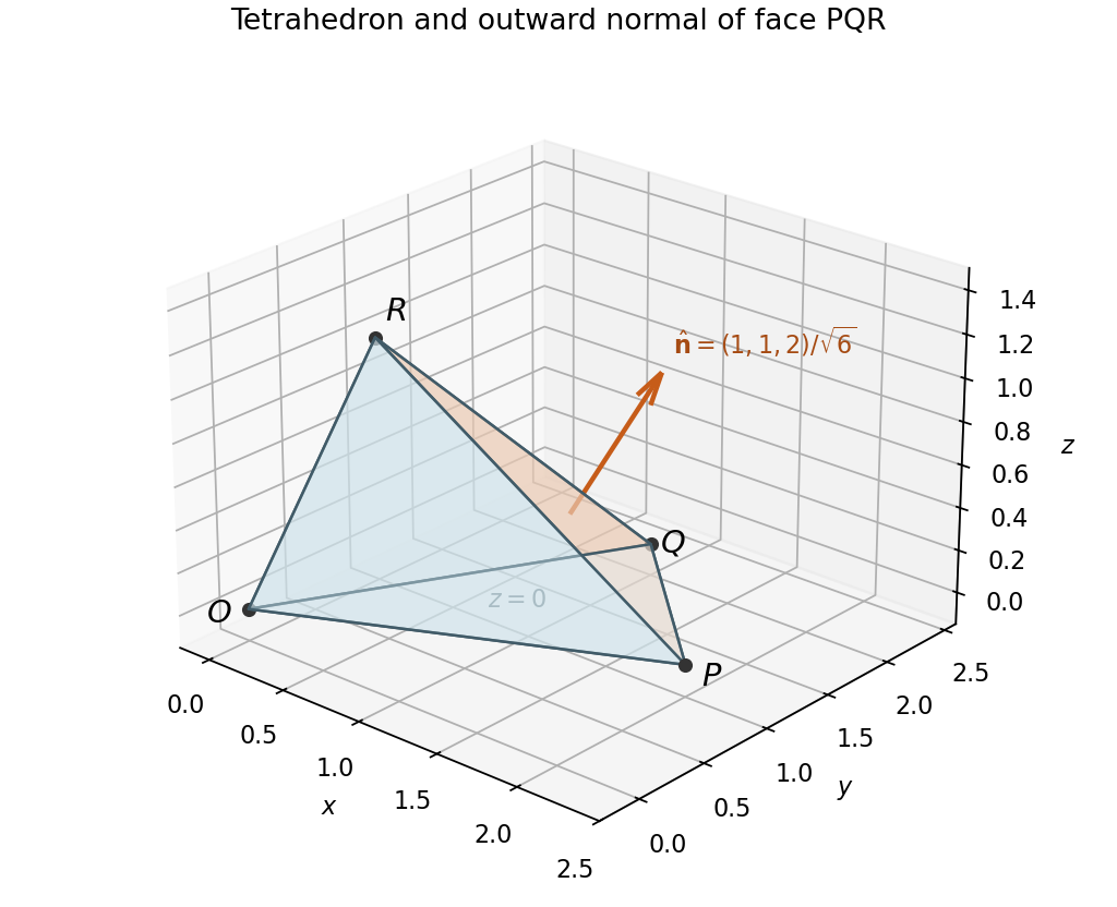
Figure 1.
Tetrahedron with its highlighted face PQR and outward unit normal
. Details. 
The normal from (ii) gives the plane equation . The distance from a point to a plane is the absolute value of the normalized plane equation at that point. At the origin this givesFor a geometric check, the perpendicular foot is , parallel to the normal and satisfying the plane equation. Its Euclidean norm is the same distance.
The volume of a parallelepiped is the absolute scalar triple product of its three edge vectors. Since ,The factor appropriate to a tetrahedron must not be applied to this parallelepiped.
Inside the sphere, the electric field has the form , including at the origin. Thus it is a conservative vector field. Outside, use the gradient of a radial function to obtainThis is also an explicit potential of a conservative vector field, single-valued throughout the exterior region. Equivalently, the curl vanishes in both regions: for a radial coefficient , because is radial. The interior formula avoids any apparent issue at the origin. The vector-field potentials here have the opposite sign from the electric potential convention used in (b).
For a radial electric potential, . Comparing radial coefficients givesIntegrating these one-variable derivatives gives the general local expressionsThe two constants are initially independent because these integrations were performed in separate radial regions.
The condition at infinity gives . Matching the electric potential at givesConsequentlyThis function is finite and differentiable at the origin. At the joining radius, both and match, giving and . Thus the electric field is continuous there as well as being conservative on each side. This is the potential of a uniform spherical source, with source coefficient .
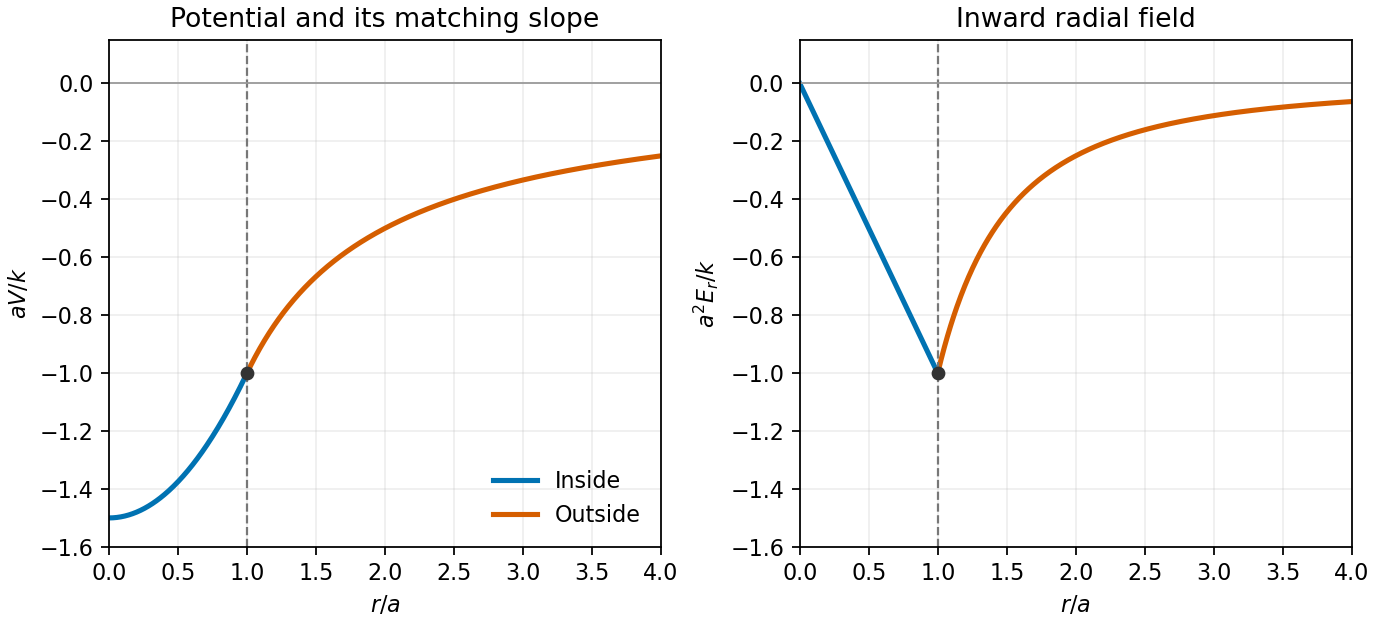
Continuous radial potential and inward electric field, normalized at the sphere boundary
. Details. 
The multivariable chain rule givesSubstituting the three parametrizing functions also writes the complete derivative asAt , the point is , its velocity is , and . Hence
Write the differential one-form as . An exact differential form must satisfy equality of mixed partial derivatives, . HereEquality at every holds precisely when . Since these polynomials are smooth on the simply connected plane, the closed-form condition is also sufficient for exactness; the explicit potential of a conservative vector field constructed in (c) verifies that sufficiency directly.
With , integrate the coefficient with respect to :Its other partial derivative is . Matching the coefficient gives . Therefore the differential equation is , and its implicit general solution isThese are level curves of the potential of a conservative vector field. Where , they give the usual graph solution . At , the implicit description retains possible vertical tangents instead of dividing by zero.
A cubic version of Taylor's theorem requires the corresponding higher differentiability, rather than only one derivative. For example, if has four continuous derivatives on the interval between and , thenwhere the Lagrange form of the Taylor remainder isfor some strictly between and when they differ. At , the remainder is zero. These hypotheses apply to both functions used below.
The required derivatives are , , , and . The four-term Taylor polynomial about one, evaluated at two, isThe Taylor remainder is for some . ThusIts negative sign also shows that this approximation is an overestimate. Bounding the fourth derivative throughout the interval establishes the requested error estimate without using a decimal value of .
Factor . This givesThe last function is even. Its Taylor series begins , since and . ThereforeIn particular, the cubic coefficient is zero; the identity explains its cancellation before any lengthy differentiation.
There are eighteen equally likely first choices. Counting the relevant subsets givesFor conditional probabilities, restrict the denominator to the conditioning subset:The five counts come from the same finite sample space, so no independence assumption is involved.
Insert the values from (a) into Bayes' theorem:Thus the identity is satisfied. Equivalently, both and equal the joint probability .
Condition on whether the first selection was a red apple. Its probability is . If it was, two red apples remain among seventeen fruits; otherwise three remain. The law of total probability givesThe same result follows from exchangeability: before either selection is observed, each ordered draw position has the original red-apple fraction , despite dependence between the draws.
Let denote a green pear on the first draw and a red apple on the second. The two categories are disjoint, so after there are still three red apples among seventeen remaining fruits. Thus . Using from (c), conditional probability givesEquivalently, conditioning on the second fruit being one particular category removes a red apple and leaves the other seventeen fruits symmetrically eligible for the first position.
The Leibniz integral rule accounts for both the moving upper endpoint and the integrand's dependence on :For the specified integrand this gives . When , integration by parts givessoFor the requested independent check, direct integration gives at . Its derivative is , agreeing with the result above. At zero the apparent singularity is removable: , so .
For ,In particular its absolute value is bounded by , proving convergence when ; the apparent endpoint singularity at one is removable, with value . On any compact parameter interval with lower bound , the differentiated integrand is , dominated by . The dominated convergence theorem therefore justifies differentiation under the integral sign:Hence . Since the integrand is identically zero at , fixes . ThusThis proves the logarithmic integral representation of the natural logarithm, including its parameter range.
Write the kernel as , with . Its partial derivatives areThus the heat kernel itself satisfies . The proposed convolution consequently givesThis verifies the heat equation. The parameter is positive time; the real integral formula is not defined at negative time.
The passage of derivatives through the integral needs justification. A sufficient condition is the Gaussian-weighted absolute integrability in heat-kernel convergence for Gaussian-integrable initial data; it holds, in particular, for data of polynomial growth. On compact positive-time intervals strictly below an integrable later time, the differentiated kernels have an integrable Gaussian bound, so differentiation under the integral sign applies.
Even if the PDF's assumed convergence is read as ordinary conditional convergence, one can justify the same calculation. Choose a later time and let be a primitive of . Convergence at spatial point zero and time makes bounded on both tails. Put . This function, its spatial and time derivatives, and their -derivatives decay as Gaussians when . Integration by parts rewrites the convolution as , with vanishing endpoint terms. Boundedness of now permits differentiation under this absolutely convergent integral; since , the same equation follows. Thus one need not silently equate conditional and absolute convergence.
Articles were limited to the first 100 out of 103 total.
Articles by others on the same topic
There are currently no matching articles.