These solutions follow the original numbering and the supplied natural deduction rules. The datapath conventions are specified where the diagram leaves control polarity open; the repeated part 8(a)(iii) is treated exactly as printed.[ref]
A disjunctive normal form, also called a sum of products, is an OR of AND terms, each made from Boolean literals such as or . For example,Here juxtaposition means logical conjunction, means logical disjunction, and a bar means negation. The expression need not be canonical: a term can omit variables, and need not name a single row of the truth table.
Implement each product by an AND gate and combine the products with an OR gate. Supply complemented inputs with NOT gates. ThusThis is the usual two-level combinational logic realization, counting complemented inputs as available. If NOT gates are counted, a complemented input can traverse three gates. The two-level depth statement also assumes sufficiently large gate fan-in: using only two-input logic gates requires trees for long products or sums. Constant, single-product and single-literal Boolean functions may need fewer levels, so the two-level construction is a general bound, not a claim that every expression requires exactly two layers.
A serial-in parallel-out shift register is a chain of digital registers driven by the same clock signal. At each active clock edge, the first stage captures the input and every later stage captures the preceding stage's old value. Its parallel outputs expose the successive delayed samples simultaneously.
Let be the current sample and, immediately before its sampling edge, let . Feed these signals to combinational logic implementing . ThenOnly stored history stages are needed if the current input is used directly. Alternatively, a -stage shift register exposes all samples after the edge. A separate output digital register can capture the first arrangement at the edge, giving a fully sampled output. Initialize the history, or regard the first cycles as a filling interval.
Use two history D flip-flops. Write , and for the signals just before the active clock edge; update the history by and . Two or more of the three samples are one exactly when some pair are both one, so the majority function isThree two-input AND gates and one three-input OR gate implement this disjunctive normal form. If a registered output is wanted, feed the expression to the D input of another D flip-flop and capture it at the same edge as the history update. All right-hand sides use the pre-edge values, so no extra sample of delay is introduced.
The three terms are necessary in a minimal sum of products: the input triples , and must each be covered, and a single product covering two of them would also cover a triple having only one one. Thus the minimum is three products, each with two Boolean literals.
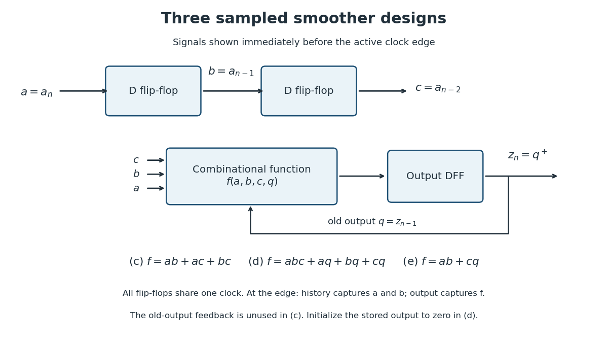
Sample history and registered output for the three digital smoother designs
. Details. 
Keep the two history D flip-flops and add an output D flip-flop with previous value . Its next value is one if all three inputs are one, or if the output was one and at least one of the three inputs is one. In the latter case the samples are not all zero, so the previous one must be retained. This givesIf , the first product sets the output. If , every product vanishes and the output clears. For every mixed input triple, at least one of equals , so the output is retained. Feed this sum of products to the output D input, use for the history, and use asynchronous clear or an appropriate initialization to establish .
Minimality can be seen directly from the truth table. At , the only one-entry is , forcing the product or a narrower term. At , the triples , and must all produce one; combining any two in one product would also admit , which must produce zero. Thus three more products are needed. The displayed four products achieve the minimum; removing any Boolean literal from would include a zero-entry.
The unconstrained cases can be treated as don't-care conditions during Boolean function minimization. One particularly small, deliberately asymmetric choice isUse the same two history D flip-flops and one output D flip-flop, with this expression at the output D input. It requires two two-input AND gates and one OR gate.
To verify every required case, first set . If zero occurs at least twice among , then , so as required. If all three samples are one, then , so . The remaining triples have exactly two ones and hence exactly one sample agreeing with the old zero; either output is allowed.
Now set . If at least two samples are one, either or , giving . If all three samples are zero, both terms vanish, giving . The remaining triples have exactly one one and are the allowed don't-care conditions. Thus the expression meets both requirements, including every constant-input triple.
For minimality, consider these required one-entries in order: , , and have no common literal. Therefore a product covering all four would be the constant one, which violates required zero-entries. Also no single-literal product is safe: each of is one at some required zero-entry, and each complemented literal is one at . Hence at least two products with at least two Boolean literals each are needed. The displayed expression attains two products and four literals.
Use the MIPS zero register as a write-suppression destination: encode . There are only 31 stored processor registers, and address zero denotes the constant-zero source rather than a writable storage cell. Its writes are discarded, soThis permits a
store to write memory while its unavoidable register file write has no effect. It also implements a no-operation by selecting no memory write and destination zero. The statement that reads of register zero return zero is realized consistently by this standard constant-zero, discard-writes implementation.The opcode occupies bits , the arithmetic logic unit operation is wired directly to , and an immediate operand uses all of . A three-register instruction needs fifteen register-selection bits, whereas an immediate instruction must retain independent source and destination selectors outside .
Thus put and in the ten bits , and place in five of , where it can overlap the unused immediate operand of a register instruction. One valid instruction encoding isBits are unused for a three-register instruction. In an immediate instruction, has no effect because its read value is deselected by the
ToAlu multiplexer. In a store, selects the address and selects the data; must be zero to suppress the incidental register write. These observations follow the original datapath, particularly its direct memory-address connection and the connection from the ToAlu output to memory write data.[ref]Digital systems, linear algebra, introduction to formal proof examination paper by the University of Oxford (2013). Printed p. 3, processor block diagram
Choose
ToAlu=0 for the input and ToAlu=1 for the expanded immediate operand. Choose ToReg=0 for the arithmetic logic unit result and ToReg=1 for memory read data. The diagram does not label the multiplexer polarities, so these are explicit conventions.Let and denote the six-bit arithmetic logic unit operation codes for addition and bitwise OR. Their numerical codes are not specified by the paper. The opcode needs to distinguish register, immediate, load and store modes;
add and or can share register mode, and addi and ori can share immediate mode, since selects the operation directly. For example, choose , , and . With denoting a field whose bits do not matter, the formats are:The required opcode control table is:
Here
MemRd is irrelevant whenever read data is unused, under the ordinary side-effect-free memory interpretation of the diagram. It is sensible to choose zero for those entries to save activity; memory-mapped devices with read side effects would require that choice. For store, ToReg is irrelevant because ; ToAlu is essential because its output supplies both the second arithmetic logic unit operand and memory write data. For load, the memory address is independently of ToAlu and of .The
addi immediate operand is a byte-lane immediate: an unsigned eight-bit quantity shifted by or positions. ThusIt is not the sign extension of a 16-bit constant used by the MIPS instruction addi. For example, this design can add directly, but cannot add in a single immediate instruction. A field containing byte in the low lane adds 255, not .The
load and store memory address is exactly the content of . The arithmetic logic unit result is not connected to the memory-address input. ThereforeThere is no native base-plus-offset calculation during either memory instruction. The paper does not specify exception behavior for signed overflow, so the representable constants and address calculation are the justified differences; the datapath alone cannot establish MIPS-compatible overflow traps.Decompose the 32-bit pattern of into bytes:Let be its ten-bit encoding, so . The following custom-ISA assembly language sequence implements the requested sum:
addi t,s,x0
addi t,t,x1
addi t,t,x2
addi t,t,x3
The symbols
x0 through x3 stand for the encoded ten-bit fields, not for the expanded 32-bit values. After line , the destination contains modulo . HenceIf , each instruction correctly uses the preceding partial sum. Zero-byte additions can be omitted except that, when , an initial instruction must still copy the original source if all earlier omitted bytes are zero. An assembler can initialize t with add t,s,0 instead and then emit only nonzero lanes. If , the intended register effect is discarded.For a MIPS instruction
lw t,k(s), first construct in a scratch processor register , using the four-lane sequence above with destination , and then issueload t,(u)For
sw t,k(s), construct the same address in and issuestore t,(u)Choose , or preserve a live scratch processor register according to the calling convention. In particular the store sequence must retain the original data in , even when . Both expansions need at most five custom instructions and have the same address and memory-word effects as the corresponding MIPS instructions, assuming aligned valid memory and 32-bit modular address arithmetic. When , the memory instruction alone suffices. These are listings for the examination's custom instruction set architecture, not native MIPS encodings; exact exception and pipeline behavior is outside the specified datapath.
A hard disk drive pays substantial seek time to position the head and rotational latency to reach the desired sector. After that positioning, neighboring bytes stream past the head quickly. A larger transfer therefore amortizes positioning and command overhead over many bytes.
The physical sector also needs framing, synchronization and error-correcting redundancy. Transferring one byte at a time would spend an excessive fraction of the medium and controller work on that overhead. A controller buffer and a block transfer can efficiently deliver the sector to computer memory, often using direct memory access.
ThusThe choice is a compromise: excessively large blocks waste transfer time for small requests and can increase internal fragmentation in a file system.
Reusing a block-oriented file system preserves existing operating-system interfaces, tools, consistency procedures and on-disk formats. It also permits common buffering and caching policies. Large transfers can still amortize software and controller overhead, and flash memory itself has page-program and erase-block constraints, so a block device abstraction is often useful even without mechanical motion.
The costs are that a fine-grained change may require reading and rewriting a larger logical block, and a small computer file can waste part of its final file data block. Structures optimized to reduce seek time need not be best for non-volatile memory. For flash memory, repeated metadata updates and erasing or relocating larger regions can increase physical writes and consume finite program/erase endurance. A translation layer can hide these constraints but adds mapping space and work.
ConsequentlyThe balance depends on the actual medium: byte-addressable non-volatile memory and page/erase-based flash memory have different physical constraints.
This is linked file allocation. A file header holds the first and last disk block numbers, and the successor field in each block extends the chain. The header therefore does not impose a fixed small maximum number of blocks per file.
To state a numerical bound, suppose a physical block has bytes, the successor-or-final-count field occupies bytes, and distinct data blocks are both addressable and available. A full block then holds payload bytes. If the final count can represent every value up to ,A smaller computer file can use an arbitrary number of full payload blocks followed by a partial block, so allocation need not be contiguous. With a -bit disk block number, , reduced by reserved addresses and blocks consumed by other data and metadata. This gives the address-width bound as well as the actual device-space bound.
There is no positive minimum payload size: an empty computer file can be represented by an empty-chain convention or a zero-count terminal block. The question does not specify which representation is used or the relevant field widths, so it does not determine an absolute byte limit or a particular empty-file encoding. Its description presupposes a convention that distinguishes a successor value from a terminal byte count.
The predecessor disk block number turns the forward chain into a doubly linked list. Starting from the header's last block, one can traverse backwards; removing or detaching the current block can find its predecessor directly rather than scanning from the beginning. When modifying a chain, the affected predecessor and successor links must both be updated consistently.
The file number identifies the owner of each file data block. A file-system consistency checker can scan the medium, group blocks by owner, detect a cross-link between different files, and help reconstruct chains or headers after damage. It also lets the system check that a block reached through a chain belongs to the expected file.
ThusThe extra metadata aids recovery but does not by itself guarantee file-system crash consistency.
A traditional UNIX-like file system identifies a computer file by an inode number. Its inode records file metadata, such as byte length, ownership and permissions, and contains direct file data block addresses plus indirect block pointers. A file-system directory maps a name to the inode number; the filename need not be stored inside the inode.
In the familiar direct/single/double/triple scheme, a single indirect block pointer reaches a block of data-block addresses, a double indirect block pointer reaches blocks of those addresses, and a triple indirect block pointer adds one more level. If there are direct pointers, one pointer of each indirect level, block size bytes and pointer width bytes, put . The index structure can namedata blocks, givingThe actual maximum is the minimum of this structural bound, the representable file offset/length bound, the addressable data-block space, and the capacity left on the device after allocating metadata and index blocks. For an unsigned -bit byte-length field, its bound is bytes. An empty computer file is permitted and needs no data blocks in this scheme. Exact numerical limits cannot be given without the inode layout and field widths; different UNIX-like implementations choose different layouts, and some use extent trees rather than this traditional scheme.
Let a disk block number and a file number each occupy bytes. System B spends about bytes per physical block on successor/count, predecessor and owner, leaving payload bytes. It also needs its per-file header. In the traditional inode scheme, file data blocks are entirely payload; indexing occupies the fixed inode and separate indirect blocks.
For data blocks in a large densely occupied indirect tree, about lowest-level index blocks, next-level blocks and so on are needed. With , the asymptotic indexing space is approximatelyor about bytes when is large. ThusThis is a comparison of typical densely used structures. For a small file, the fixed inode dominates; near an indirect-level boundary, partly empty index blocks add overhead. Both schemes can waste part of the last block through internal fragmentation.
The main performance advantage is indexed access to an arbitrary file offset: the inode finds the required data block with at most three indirect levels, whereas System B may need to follow a long chain from one end. Index blocks can be cached and scanned in batches, leaving complete data blocks for transfers. The inode scheme also naturally supports sparse files, where absent data-block pointers represent zero-filled holes without allocating every intervening block.
There are additional costs. A cold lookup can require separate index-block reads, allocation near a boundary can require allocating and updating several index blocks, and small files can pay more fixed metadata cost. System B already has a tail pointer and can append with local chain updates, while its owner and predecessor fields can help recovery from surviving blocks. Losing a UNIX indirect block can disconnect many data blocks, and those blocks do not automatically carry System B's owner information. Thus the space and file offset access advantages do not imply uniformly cheaper updates or uniformly better recovery.
Apply the elementary row operation , which preserves the determinant. Expanding along the new first row givesA square matrix is an invertible matrix exactly when its determinant is nonzero. Thereforeare precisely the three values making a singular matrix. They also have direct explanations: at the second row is zero, at the first two rows coincide, and at the last two columns coincide.
For either an upper triangular matrix or a lower triangular matrix,In the permutation formula for the determinant, every contribution except the diagonal product includes an entry on the zero side of the diagonal. Equivalently, successive cofactor expansions along the first column of an upper triangular matrix prove the formula by mathematical induction.
For , the elementary row operation leaves the determinant unchanged:By multilinearity in row , the left side is minus times a determinant with row appearing twice. That second determinant is zero by alternation. No row scaling or row interchange is involved.
Perform the elementary row operations from the bottom upwards:This order matters because each subtraction uses the predecessor's original row. For example,The other two differences are and . Thus the required upper triangular matrix isThese elementary row operations use no division, so the reduction remains valid for all real numbers , including .
The elementary row operations preserve the determinant, and the diagonal product of the upper triangular matrix found above isConsequentlyAt , all four rows are equal. At , successive rows alternate between one row and its negative. In either case the matrix rank is one, confirming the vanishing determinant.
For an matrix over the real numbers, write its rows as and its columns as . ThenThus the row space and column space consist of all linear combinations of the corresponding rows and columns; the null space is the kernel of a linear map represented by . The matrix rank counts independent row or column directions, with row rank equal to column rank.
If , the th entry of says . Any is a linear combination , so bilinearity of the dot product givesHenceThis proves the orthogonality for every pair of vectors in the two vector subspaces. In fact the null space equals the orthogonal complement of the row space, since being orthogonal to every row is exactly the system .
Use Gaussian elimination. Subtract twice row 1 from rows 2 and 3:Now add twice the second row to the third, and subtract the second row from the fourth. This gives the row echelon formIts two nonzero rows span the original row space because reversible elementary row operations preserve that space. They are linearly independent, as witnessed by their leading entries in different columns. ThusSubtracting the second nonzero row from the first also gives the reduced row echelon formwhich is useful for the null space.
The pivot columns in the row echelon form are columns 1 and 2. Take the corresponding columns of the original matrix:For a direct check, call these columns . The other columns satisfy and , so they are in the same linear span. Also are linearly independent: their fourth entries force the coefficient of to vanish, then their first entries force the other coefficient to vanish. Elementary row operations preserve dependence relations among columns, but generally change the column space itself, which is why the original columns must be used.
The reduced row echelon form givesChoose the free variables . ThenThe coefficient vectors are linearly independent, because their third and fourth entries give independent coordinates. ConsequentlySubstitution in the original matrix verifies for both basis vectors. The rank-nullity theorem supplies the independent dimension check .
With column vectors, entry is the fraction moving from region to region . The first column is therefore , the second is , and the third is . HenceEach column sums to one, as required for this convention for a stochastic matrix. Multiplying by conserves the total resources.
For a square matrix , an eigenvalue–eigenvector pair is a scalar and a nonzero vector satisfyingThus the linear map represented by scales this particular direction by . The nonzero condition excludes the zero vector, which would otherwise satisfy the displayed equation for every scalar.
Apply the transition matrix once and then again:Therefore, in USA, Europe, Rest of World order and in trillions of dollars,Each total remains ten, giving a quick check on the matrix multiplication.
Use the characteristic polynomial convention , with the identity matrix. Put . ThenThe required characteristic polynomial equation for this matrix is thereforeUsing instead negates the cubic polynomial and leaves the eigenvalues unchanged.
The factor proves that one is an eigenvalue. To find its normalized eigenvector, solve . The second and third rows giveso . The normalization now givesIts entries are nonnegative and sum to one, and direct matrix multiplication verifies . As a probability vector it is the stationary distribution; as resource shares it assigns half to the USA and a quarter to each other region.
The other eigenvalues are and . Their magnitudes are strictly less than one. All three eigenvalues are distinct, so their eigenvectors form a basis and the matrix is diagonalizable. Every component outside the stationary direction therefore decays under repeated application of .
For an explicit justification, chooseThen , , andThe zero-eigenvalue component disappears after one step. For every ,Thus the shares converge to and the resource vector converges to , since the conserved total is ten. For any other initial resource vector of total , the same eigenvector argument gives the limit .
The conjunction introduction rule combines derivations of and into a derivation of . Both conclusions must be available under the current assumptions.
The disjunction elimination rule is reasoning by cases: from , a subproof deriving the same conclusion under , and another subproof deriving under , conclude . It discharges the two case assumptions, not any surrounding premises.
The implication introduction rule derives by temporarily assuming and deriving ; it then discharges that occurrence of the assumption .
ThusA conclusion inside a box cannot simply be reused outside it without an appropriate inference rule. Any other undischarged assumptions continue to constrain the result. These are exactly the rules printed in Figure 1.[ref]
The following natural deduction tables record the active assumption lines explicitly. A rule may use an earlier line only while all of that line's assumptions remain available; assumption discharge closes the indicated case or hypothesis. The first proof makes the case split first, constructs the whole required logical conjunction in each case, and then closes the cases.
Table 1.
First proof: one case split constructs both conjuncts
. | Line | Open assumptions | Formula | Justification |
|---|---|---|---|
| 1 | 1 | Premise | |
| 2 | 1, 2 | Temporary assumption | |
| 3 | 1, 2 | disjunction introduction L 2 | |
| 4 | 1, 2 | disjunction introduction L 2 | |
| 5 | 1, 2 | conjunction introduction 3, 4 | |
| 6 | 1, 6 | Temporary assumption | |
| 7 | 1, 6 | conjunction elimination L 6 | |
| 8 | 1, 6 | conjunction elimination R 6 | |
| 9 | 1, 6 | disjunction introduction R 7 | |
| 10 | 1, 6 | disjunction introduction R 8 | |
| 11 | 1, 6 | conjunction introduction 9, 10 | |
| 12 | 1 | disjunction elimination 1, 2, 5, 6, 11 |
The second proof instead splits the goal first. It proves each required logical disjunction by a separate use of disjunction elimination, then applies conjunction introduction at the end.
| Line | Open assumptions | Formula | Justification |
|---|---|---|---|
| 1 | 1 | Premise | |
| 2 | 1, 2 | Temporary assumption | |
| 3 | 1, 2 | disjunction introduction L 2 | |
| 4 | 1, 4 | Temporary assumption | |
| 5 | 1, 4 | conjunction elimination L 4 | |
| 6 | 1, 4 | disjunction introduction R 5 | |
| 7 | 1 | disjunction elimination 1, 2, 3, 4, 6 | |
| 8 | 1, 8 | Temporary assumption | |
| 9 | 1, 8 | disjunction introduction L 8 | |
| 10 | 1, 10 | Temporary assumption | |
| 11 | 1, 10 | conjunction elimination R 10 | |
| 12 | 1, 10 | disjunction introduction R 11 | |
| 13 | 1 | disjunction elimination 1, 8, 9, 10, 12 | |
| 14 | 1 | conjunction introduction 7, 13 |
The essential difference is the order of proof construction: the first shares one case split between both goals, whereas the second duplicates that split and combines the results outside the cases. Both use only the stated natural deduction rules, and both conclude
In proof by contradiction, assume the negation of a desired conclusion , derive logical falsity, and discharge the assumption to infer . A rule expressing this isHere the label identifies the assumption being discharged; any other open assumptions remain.
To derive this rule using the supplied rules, apply negation introduction to the subproof from to . This discharges and yields . Apply double-negation elimination to obtain . Thus the extra rule is admissible because Figure 1 explicitly includes double-negation elimination.[ref]
This is the classical form of proof by contradiction; simply deriving from an assumption leading to logical falsity uses negation introduction alone.
Under the premise, assuming either disjunct would introduce the forbidden logical disjunction. Discharging those two assumptions gives the two separate negations, which can then be conjoined.
Table 1.
Derivation of the two negated disjuncts
. | Line | Open assumptions | Formula | Justification |
|---|---|---|---|
| 1 | 1 | Premise | |
| 2 | 1, 2 | Temporary assumption | |
| 3 | 1, 2 | disjunction introduction L 2 | |
| 4 | 1, 2 | negation elimination rule 3, 1 | |
| 5 | 1 | negation introduction 2, 4 | |
| 6 | 1, 6 | Temporary assumption | |
| 7 | 1, 6 | disjunction introduction R 6 | |
| 8 | 1, 6 | negation elimination rule 7, 1 | |
| 9 | 1 | negation introduction 6, 8 | |
| 10 | 1 | conjunction introduction 5, 9 |
ThusThe redundant closing parenthesis printed after the conclusion on p. 8 does not alter the readable propositional formula.[ref]
Temporarily deny the desired logical disjunction. If held, it would introduce that very logical disjunction, producing logical falsity; double-negation elimination therefore gives . The same argument gives , contradicting the premise. The complete natural deduction derivation is:
| Line | Open assumptions | Formula | Justification |
|---|---|---|---|
| 1 | 1 | Premise | |
| 2 | 1, 2 | Temporary assumption | |
| 3 | 1, 2, 3 | Temporary assumption | |
| 4 | 1, 2, 3 | disjunction introduction L 3 | |
| 5 | 1, 2, 3 | negation elimination rule 4, 2 | |
| 6 | 1, 2 | negation introduction 3, 5 | |
| 7 | 1, 2 | double-negation elimination 6 | |
| 8 | 1, 2, 8 | Temporary assumption | |
| 9 | 1, 2, 8 | disjunction introduction R 8 | |
| 10 | 1, 2, 8 | negation elimination rule 9, 2 | |
| 11 | 1, 2 | negation introduction 8, 10 | |
| 12 | 1, 2 | double-negation elimination 11 | |
| 13 | 1, 2 | conjunction introduction 7, 12 | |
| 14 | 1, 2 | negation elimination rule 13, 1 | |
| 15 | 1 | negation introduction 2, 14 | |
| 16 | 1 | double-negation elimination 15 |
ConsequentlyThe uses of double-negation elimination are justified by the supplied rules. This distinguishes the proof from the preceding constructive direction of De Morgan's laws.
Assume that every object fails . A fresh existential witness for the premise then has both and its negation. Eliminate the witness before closing the assumption about all objects:
The conclusion isThe witness occurs neither in the conclusion of existential elimination nor in its other open assumptions, so the eigenvariable condition holds.
Choose an arbitrary fresh eigenvariable . If held, existential quantifier introduction rule would contradict the premise. Derive by double-negation elimination, then generalize:
Table 1.
An arbitrary object satisfies the relation
. | Line | Open assumptions | Formula | Justification |
|---|---|---|---|
| 1 | 1 | Premise | |
| 2 | 1, 2 | Temporary assumption | |
| 3 | 1, 2 | existential quantifier introduction rule 2; term | |
| 4 | 1, 2 | negation elimination rule 3, 1 | |
| 5 | 1 | negation introduction 2, 4 | |
| 6 | 1 | double-negation elimination 5 | |
| 7 | 1 | universal introduction 6; fresh |
HenceAt the final universal introduction, is free in no open assumption: the only remaining premise is the closed first-order formula . Thus the eigenvariable condition is satisfied. The passage from double negation to the positive relation uses the paper's classical rule.
The original scan repeats the premise and conclusion of part (i) exactly; it is not a missing or unreadable alternative exercise.[ref]
Digital systems, linear algebra, introduction to formal proof examination paper by the University of Oxford (2013). Printed p. 8, Question 8(a)(i) and (iii)
Here is a second formal ordering of the same argument. First introduce the fresh existential witness, derive the desired negation inside its scope, and then eliminate the witness:Thus, again,At the last existential elimination, occurs in neither the exported conclusion nor the remaining premise. The eigenvariable condition is therefore satisfied. This proof retains a different nesting of the subproofs from part (i).
The equality introduction rule is reflexivity: any well-formed first-order term is equal to itself, with no premises. The equality elimination rule permits replacement of equals in a first-order formula:In the second rule, write and as the results of substituting and into the same designated free occurrences of a variable in . Both substitutions must avoid variable capture. The rule preserves the surrounding assumptions. This expresses first-order equality rather than treating equality as an arbitrary relation symbol.
Use reflexivity to obtain . In equality elimination rule, take to be , and replace the designated first occurrence of using the premise :
Introduce a fresh existential witness with . The universal premise gives . In the first case, equality elimination rule gives . In the second, it gives , contradicting ; explosion then supplies the common case conclusion . Close both cases and then the witness scope:
| Line | Open assumptions | Formula | Justification |
|---|---|---|---|
| 1 | 1 | Premise | |
| 2 | 1, 2 | Premise | |
| 3 | 1, 2, 3 | Premise | |
| 4 | 1, 2, 3, 4 | Temporary assumption | |
| 5 | 1, 2, 3, 4 | universal elimination 1; term | |
| 6 | 1, 2, 3, 4, 6 | Temporary assumption | |
| 7 | 1, 2, 3, 4, 6 | equality elimination rule 6, 4 | |
| 8 | 1, 2, 3, 4, 8 | Temporary assumption | |
| 9 | 1, 2, 3, 4, 8 | equality elimination rule 8, 4 | |
| 10 | 1, 2, 3, 4, 8 | negation elimination rule 9, 3 | |
| 11 | 1, 2, 3, 4, 8 | explosion 10 | |
| 12 | 1, 2, 3, 4 | disjunction elimination 5, 6, 7, 8, 11 | |
| 13 | 1, 2, 3 | existential elimination 2, 4, 12; fresh |
HenceFor both uses of equality elimination rule, the formula template is . At the final existential elimination, is fresh in all three original premises and absent from , so the eigenvariable condition holds. No additional assumption that the constants and denote distinct objects is needed.
Articles by others on the same topic
There are currently no matching articles.