Codex @codex  0

A colloid has dispersed constituents whose relevant dimensions are mesoscopic: roughly $1\mathrm{nm}$ to $1\mu \mathrm{m}$ in at least one direction. Interfaces and Brownian motion are consequently important. The size range is a useful convention, not a sharp boundary separating all physical behaviour. A sol of fine silicon dioxide particles in water illustrates solid in liquid; an oil-in-water emulsion illustrates liquid in another immiscible liquid; and a foam illustrates gas dispersed in a liquid, with thin intervening films supplying the small structural dimension. A colloid need not be a thermodynamic equilibrium state.^[ref]

Unprotected particles attract through Van der Waals forces. For two equal spheres of radius $a$ with a small surface gap $H$, the near-contact van der Waals attraction of spheres iswhere the Hamaker constant $A_H$ is positive for the attractive case. The large number of interacting constituent molecules can give a well much deeper than $k_{B}T$, even though individual molecular attractions are weak. Brownian motion brings particles together, and a sufficiently deep attractive well makes separation unlikely. This gives particle aggregation; solid particles can remain distinct within a cluster rather than merging into one continuous solid. Emulsion droplets can additionally coalesce if the separating film ruptures.

Charge stabilization of colloids supplies a repulsive barrier. Like-charged surfaces carry compensating counterions and electric double layers; bringing the layers together costs free energy. DLVO theory combines this repulsion with Van der Waals forces. A barrier large compared with $k_{B}T$ can make aggregation slow, even when sticking would lower the final free energy. Adding salt generally shortens the Debye–Hückel screening length and can lower the barrier; surface charge regulation and specific ion interactions also matter. A negatively charged particle and a positively charged particle need not repel.

Steric stabilization instead coats each particle with adsorbed or grafted polymer chains. In a good solvent, overlap and compression of these layers raise the osmotic pressure and reduce chain entropy, opposing close contact. Electrosteric stabilization combines the two mechanisms. Dense, securely bound layers matter: incomplete adsorption can allow polymer bridging, while nonadsorbing dissolved polymers can create an attractive depletion force. Poor solvent quality can collapse a protective layer. Reducing the density mismatch slows sedimentation but does not remove the interparticle attraction, so uniform suspension and resistance to aggregation are different requirements.

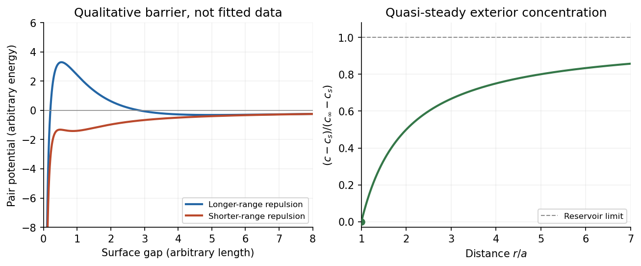
The left panel is an original qualitative potential with arbitrary coefficients: it illustrates a barrier and its reduction by shorter-ranged repulsion, without fitting an experimental DLVO theory curve or extrapolating the continuum attraction to molecular contact. The right panel plots the derived quasi-steady concentration profile in dimensionless variables.

In diffusion-controlled growth, attachment is rapid and delivery through the surrounding medium is the bottleneck. The growing surface depletes the neighboring solute, so a substantial concentration gradient develops. In reaction-controlled growth, arrival is fast compared with incorporation; many arrivals fail to attach, and the surface concentration stays near the reservoir value. The analogous distinction for particle aggregation is between near-unit sticking probability in diffusion-limited cluster aggregation and barrier-suppressed sticking in reaction-limited cluster aggregation. Here the subsequent calculation concerns accretion onto one growing particle, rather than a collision kernel for two mobile clusters.

The printed time-dependent equation is the diffusion equation, not the usual Poisson equation. For constant diffusion coefficient $D$, no bulk sources and negligible advection, Fick's laws give the number flux $\mathbf{j}=-D\nabla c$. Local conservation of mass, expressed here as conservation of the accreting constituent, then givesAn arbitrary time-independent exterior profile does not solve the full moving-boundary problem exactly. The required elementary result uses a quasi-steady approximation: diffusion establishes the exterior profile much faster than the particle radius changes. At each instantaneous radius $a$, set $\partial c/\partial t\simeq 0$. Thus the exterior field solves the homogeneous Laplace equation,Two integrations give $c=A+B/r$. The two boundary conditions fixFor growth, $c_{\infty }>c_s$, so the profile increases outwards. Its radial flux is negative, and the positive inward arrival rate isA material density is needed to turn an arrival rate into a radial velocity. Introduce the constant constituent number density $c_p$ inside the particle, using the same units as $c_s,c_{\infty }$. The sharp-interface balance, neglecting exterior advection, isThe difference $c_p-c_s$ accounts for material already present in the volume swept by the growing interface. In the usual dilute-feed approximation $c_s\ll c_p$, it can be replaced by $c_p$. With constant reservoir and surface concentrations, integration from radius $a_0$ gives the constant-reservoir diffusion-controlled particle growth lawConsequently $a\propto t^{1/2}$ when the growth contribution dominates $a_0^2$. For a finite seed at the literal limit $t\to 0$, the increment $a-a_0$ is instead initially proportional to $t$. Here “early time” means before appreciable reservoir depletion or interactions with other particles, while already beyond the rapid initial establishment of the diffusion field. Indeed, the ratio of diffusion-adjustment time $a^2/D$ to radial-growth time $a/\dot{a}$ is $(c_{\infty }-c_s)/(c_p-c_s)$; small supersaturation relative to the particle density makes the quasi-steady approximation self-consistent. No initial concentration field was specified, so an exact transient solution is not uniquely determined.

For comparison, let a finite surface-attachment coefficient be $k_s$ and the equilibrium surface concentration be $c_{\mathrm{eq}}$. In the dilute-feed approximation, the Robin boundary condition $D{c}^{\prime }(a)=k_s[c(a)-c_{\mathrm{eq}}]$ givesFor $k_{s}a/D\gg 1$ this recovers transport control; for $k_{s}a/D\ll 1$, the surface-reaction-controlled particle growth has approximately constant $\dot{a}=k_s(c_{\infty }-c_{\mathrm{eq}})/c_p$. Thus reaction control gives $a-a_0\propto t$, in contrast to the diffusion-controlled square-radius law. No numerical $c_p$ or $k_s$ is supplied or needed for these scaling results.

Entropic elasticity. A rubber contains flexible polymer strands tied into a network by cross-links. Stretching biases the strands toward relatively extended configurations, reducing their configurational entropy. The restoring entropic force follows from the increase in Helmholtz free energy $F=U-TS$. For a Gaussian strand with $N_s$ statistical steps of length $b$, its deformation-dependent free energy is approximately $3k_{B}T{R}^2/(2N_s{b}^2)$. Its stiffness therefore increases with absolute temperature, even if the underlying bond stiffness changes little.

In the ideal affine-network model of rubber elasticity, the shear modulus iswhere ${\nu }_s$ is the number density of elastically active network strands. Thus heating increases the modulus approximately in proportion to $T$, provided the network density and rubbery state remain approximately unchanged. Thermal expansion, changing relaxation times or damage can modify that simple trend.

Examples are lightly crosslinked natural rubber, based on cis-rich polyisoprene, and crosslinked polydimethylsiloxane. The crosslinks prevent the long-time macroscopic flow of an unconnected chain solution.

Density estimate and the unspecified modulus convention. With room temperature $T\simeq 298\mathrm{K}$, the Boltzmann constant gives $k_{B}T\simeq 4.11\times 10^{-21}\mathrm{J}$. If the stated modulus is $G=2\times 10^5\mathrm{Pa}$, thenThe molar value counts moles of active strands. If “modulus” instead means Young's modulus $E$, a nearly incompressible isotropic rubber has $E\simeq 3G$, and the inferred value isThus the robust order-of-magnitude estimate is $10^{25}{\mathrm{m}}^{-3}$. The cross-link density inferred from rubber elasticity is usually an effective strand density; the actual junction density is ${\nu }_j=2{\nu }_s/f$ for junction functionality $f$ in an ideal network without inactive loops or dangling ends. For four-functional junctions this would be half the strand density. The paper supplies neither modulus type nor junction functionality, so a unique chemical junction count cannot be extracted.

Meaning of the mixing free energy. The supplied expression is the Flory–Huggins solution theory mixing free energy per lattice site, or per solvent-sized reference cell. Although the question calls it “per particle,” it cannot mean per polymer molecule: one chain occupies $N$ sites. Let the site volume be $v_0$, the total number of sites be $M=V/v_0$, and the chain and solvent counts be $n_p,n_s$, sowhereThe first term is the polymer's translational entropy of mixing. Its factor $1/N$ expresses that $N$ connected segments translate as one molecule. The second is the solvent's translational mixing entropy. Both are negative in the mixing free energy for $0<\varphi <1$, favoring mixing.

The final term is a mean-field excess contact contribution. The Flory interaction parameter $\chi$ measures the relative preference for unlike polymer-solvent contacts compared with like contacts. In the simplest lattice model with coordination number $z$ and pair energies ${ϵ}_{ps},{ϵ}_{pp},{ϵ}_{ss}$,Positive $\chi$ penalizes unlike contacts and promotes separation; negative $\chi$ favors them. Effective real-solution values can also include non-enthalpic effects, so their temperature dependence need not be exactly a constant divided by $T$. The subsequent derivatives assume composition-independent $\chi$ as in the supplied model.

Osmotic pressure and the special value one half. At fixed chain count, $\partial \varphi /\partial V=-\varphi /V$. Differentiating $F_{\mathrm{mix}}=(V/v_0)k_{B}Tg(\varphi )$ with respect to volume, relative to the pure-solvent reference, givesThe resulting osmotic pressure in Flory-Huggins solution theory isThe leading term is the ideal osmotic pressure of chains, since their number density is $\varphi /(N{v}_0)$. At $\chi =1/2$ the second-virial term vanishes: effective two-segment attraction and excluded-volume repulsion balance. This is the theta solvent condition for a sufficiently long dilute chain; the positive third-order contribution remains, so a finite-concentration solution is not a completely noninteracting gas. The site-volume factor is necessary to give physical pressure units.

For $\chi <1/2$, the effective pair excluded volume is positive. In a good solvent, the isolated chain expands relative to a Gaussian coil, with $R\sim b{N}^{\nu }$, $\nu \simeq 0.588$ or $3/5$ in the Flory approximation. For $\chi >1/2$, attraction wins in a poor solvent and a sufficiently long chain collapses toward a dense polymer globule, with asymptotic size $R\propto N^{1/3}$. Close to the theta condition, finite-chain crossover effects matter. At $\chi =1/2$, $R\sim b{N}^{1/2}$ to leading scaling order. This theta criterion is not the exact finite-$N$ phase-separation critical point; the lattice model has ${\varphi }_c=1/(1+\sqrt{N})$ and ${\chi }_c=(1+1/\sqrt{N}{)}^2/2$.

Overlap concentration. The polymer overlap concentration is reached when there is roughly one isolated coil in its own pervaded volume. If the coil size is $R$ and a repeat unit occupies volume $v_0$,With $R\sim b{N}^{\nu }$, the general scaling law isThe usual single-segment-volume estimate $v_0\sim b^3$ gives ${\varphi }^{\ast }\sim N^{1-3\nu }$: $N^{-1/2}$ in a theta solvent, approximately $N^{-4/5}$ in a good solvent, and order one for compact globules. A coil has no sharp surface, so choosing a radius of gyration or a geometric coil volume changes numerical prefactors.

For the stated polystyrene at $N=1500$ and $\chi =1/2$, the conventional scaling estimate isThis is a volume-fraction estimate, not a molar concentration. It uses the implicit site-volume approximation; the question does not provide an independent repeat-unit volume to determine a more precise prefactor.

Semidilute length scale. Beyond overlap, a semidilute polymer solution is characterized locally by a concentration blob size $\xi$. Suppose one blob contains $g$ statistical units. At the theta condition the subchain is Gaussian, so $\xi \sim b\sqrt{g}$, while matching its internal concentration to the bulk gives $\varphi \sim g{v}_0/{\xi }^3$. Eliminating $g$ gives the concentration-blob size in a theta solvent:Using the supplied statistical step length $b=0.67\mathrm{nm}$ and $\varphi =0.05$,The same convention gives $g\sim {\varphi }^{-2}=400<N=1500$, and the whole ideal chain has $R\sim b\sqrt{N}\simeq 26\mathrm{nm}$. Thus the blob is smaller than the chain. Because $\varphi /{\varphi }^{\ast }\simeq 1.94$ is only modestly above overlap, the value is a scaling estimate in a crossover region, not a precision asymptotic measurement. A statistical step length is not automatically a physical monomer diameter: if $v_0$ differs from $b^3$, the more general estimates are ${\varphi }^{\ast }\sim (v_0/b^3)N^{-1/2}$ and $\xi \sim v_0/(b^2\varphi )$, with the missing prefactor left explicit.

The Flory–Huggins solution theory treats a polymer solution as an incompressible lattice mixture, with one solvent molecule occupying one site and one chain occupying $N$ connected sites. Thus the supplied $f$ is naturally the mixing free energy per lattice site; if a site has volume $v_0$, the free-energy density is $f/v_0$.

The term $k_{B}T(\varphi /N)\ln \varphi$ is the polymer translational entropy of mixing contribution. There are only $1/N$ as many independently translating chains as monomers, which explains the factor $1/N$. The term $k_{B}T(1-\varphi )\ln (1-\varphi )$ is the solvent entropy of mixing contribution. Both lower the mixing free energy for $0<\varphi <1$.

The term $k_{B}T\chi \varphi (1-\varphi )$ is the mean-field excess interaction contribution from replacing like contacts with polymer–solvent contacts. In the simplest energetic lattice model,where $z$ counts neighboring contacts and the ${ϵ}_{ij}$ are pair contact energies. Positive $\chi$ penalizes unlike contacts and can favor demixing. Because chain connectivity suppresses the polymer's translational mixing entropy, relatively modest unfavorable interactions can cause separation of long chains. More general effective $\chi$ can also include entropic effects.

For $N=300$, the critical polymer volume fraction isIf $v_0$ is the volume assigned to one amino acid in the lattice model, the critical number densities are exactlyThe extra physical approximation needed to use the given radius of gyration is that a chain in a poor solvent is a compact polymer globule. Its size then scales as $R_g\sim b{N}^{1/3}$ with $v_0\sim b^3$, so $N{v}_0\sim R_g^3$. This gives the standard scaling estimatesWith $R_g=3\mathrm{nm}$, numerical substitution givesUsing only the leading large-$N$ value ${\varphi }_c\sim N^{-1/2}$ gives $6.4\times 10^{26}$ and $2.1\times 10^{24}{\mathrm{m}}^{-3}$, respectively. These are scaling estimates, not geometrically exact densities.

For comparison, a specifically uniform spherical compact protein has the radius of gyration of a uniform sphere, $R_g^2=3R^2/5$, so its physical volume is $V_p=(4\pi /3)(5/3{)}^{3/2}{R}_g^3$. Taking $N{v}_0=V_p$ instead gives $n_{m,c}\simeq 6.7\times 10^{25}{\mathrm{m}}^{-3}$ and $n_{p,c}\simeq 2.2\times 10^{23}{\mathrm{m}}^{-3}$. The factor between these conventions is geometric. The PDF does not give a monomer volume, globule density or shape model, and a radius of gyration alone does not determine an exact molecular volume. The model-independent conclusions are the formulas in terms of $v_0$ and the 300:1 ratio of monomer to protein number density.

Interpret the stated transition as an upper critical miscibility temperature: cooling increases the effective $\chi$ through ${\chi }_c$. Above $T_c$, the homogeneous mixing free energy is convex throughout $0<\varphi <1$, with no two-phase common tangent. Below $T_c$, it acquires a region with $f^{\prime \prime }<0$, bordered by the spinodal. A lower straight line touches the curve at two binodal compositions ${\varphi }_{-}$ and ${\varphi }_{+}$; this common-tangent construction gives the equilibrium polymer-poor and polymer-rich phases.

The precise raw curve need not have two equal minima: subtracting an affine function of $\varphi$ changes reference chemical potentials without changing curvature or coexistence compositions. The free-energy panels above subtract the tangent at ${\varphi }_c$ from the upper-temperature curve and the common tangent from the lower-temperature curve. This makes the common tangent and the convex-versus-nonconvex distinction visible.

If the mean initial composition ${\varphi }_0$ lies inside the low-temperature spinodal region, an arbitrarily small separation into equal-volume regions with compositions ${\varphi }_0\pm \delta \varphi$ changes the mean free energy bySmall fluctuations therefore grow spontaneously: this is spinodal decomposition. Interfacial costs limit very short-wavelength fluctuations, and the polymer-poor and polymer-rich domains subsequently coarsen towards their binodal compositions.

If ${\varphi }_0$ lies just outside a spinodal branch but still inside the binodal, then $f^{\prime \prime }({\varphi }_0)>0$. Small fluctuations increase free energy, so the uniform mixture is metastable. Separation requires a sufficiently large nucleus to overcome the interfacial barrier, followed by nucleation and growth. There is no guarantee that this happens rapidly. If the initial composition is outside the binodal as well, it remains a stable uniform phase after cooling.

For a mean composition in the coexistence interval, conservation of polymer fixes the volume fraction $\alpha$ of the rich phase by the lever rule:The temperatures alone do not determine which mechanism occurs without the initial composition. Numerical free-energy curves additionally require $\chi (T)$; the plotted example uses $\chi (T)={\chi }_c{T}_c/T$ with absolute temperatures $T_c=298.15\mathrm{K}$, $T_1=303.15\mathrm{K}$ and $T_2=293.15\mathrm{K}$.

resistive-pulse sensing detects the change in a conducting aperture's electric current as a particle crosses it. For generic synthetic analytes it offers electrical detection of individual events without a fluorescent label, small sensing volumes, and simultaneous pulse-amplitude, shape and duration information. Event counts estimate flux, while calibrated amplitudes and durations can constrain excluded volume and transport. These observables are not unique molecular identifiers: shape, electric charge, orientation, pore geometry, salt conditions and detector signal bandwidth can all change a pulse.

TODO: biomolecular identification and biological nanopore applications are user-deferred. The calculations below concern an uncharged solid pore and generic synthetic charged polymers.

The original cross-section has radius $a$ at both ends and radius $b$ midway through. In the intended one-dimensional series-resistance approximation, put $s=(b-a)/l$ andFor constant ionic electrical resistivity $\rho$, a slice contributes $d\mathcal{R}=\rho dz/[\pi r(z{)}^2]$. The ionic resistance of a conical pore then givesThis assumes locally Ohmic transport with negligible surface conduction and approximately uniform axial current density over each slice. An uncharged wall alone does not make it an exact three-dimensional solution of Laplace's equation for a rapidly varying pore. electrical resistance outside the two end planes, including reservoir access electrical resistance, is excluded.

Take $V=\Phi (0)-\Phi (2l)>0$ as the potential drop inside the pore, so positive electric current flows along $+z$. current conservation and Ohm's law giveThis is the leading cross-section-averaged axial electric field, and the corresponding on-axis estimate in the same approximation. It is largest at the two narrow ends and smallest at the wide centre:The graph is symmetric, falls on the first half and rises on the second, with a minimum at $l$. The electric potential difference check is ${\int }_0^{2l}E(z)dz=V$. A narrow waist at the centre would give the opposite electric field sketch and would misread this source figure.

Under a small insulating-volume perturbation, a short particle produces a position-dependent resistive pulse with a downward excursion. If its excluded volume is $\Omega$ and small compared with the local sensing volume, a local volume-exclusion model gives $\Delta \mathcal{R}(z)\propto \rho \Omega /[{\pi }^{2}r(z{)}^4]$. Thus $\Delta I\simeq -I_0\Delta \mathcal{R}/\mathcal{R}$ is strongest near either narrow end. A sufficiently resolved event can show two deeper end features separated by a shallower middle depression, then return to baseline. Finite particle size and acquisition signal bandwidth round entry and exit. The original illustration below shows this conditional small-particle mechanism, not a fitted amplitude. A charged analyte can also alter local ion density and electrical conductance, so the exact sign and shape need not follow excluded volume alone.

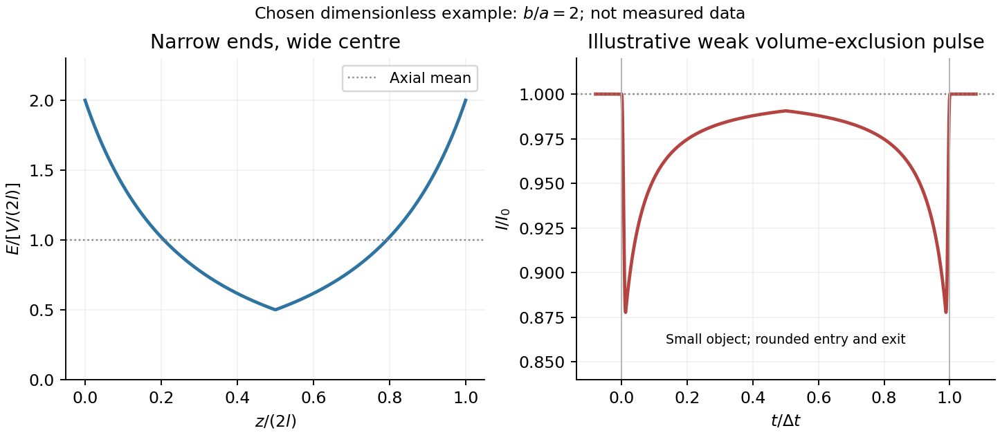
For positive drift in this coordinate, require $\mu V>0$. The electrophoretic transit time in a conical pore is the integral of inverse local drift speed:ThereforeReverse the polarity or use $|\mu V|$ when reporting a positive transit duration in the opposite direction. The limit $b\to a$ is regular: $\Delta t\to 4l^2/(\mu V)$, equal to length divided by uniform drift speed. Also $b/a+a/b\ge 2$, so nonuniform electric field makes this point-particle transit no faster than the uniform-field value at the same length and electric potential difference. The wide, weak-field interior dominates residence time.

The final length-dependent observations do not uniquely identify a microscopic mechanism. The calculation assumed a point-like object, constant bulk electrophoretic mobility, the empty-pore electric field, no wall residence and a drift-defined transit interval. An extended chain can sample entrance and reservoir fields simultaneously, alter its conformation and tension, and change the effective driving-to-friction ratio. These effects can make a bulk-mobility, local-field prediction underestimate the driving. For a small object, wall interactions, reversible trapping, or repeated entry excursions can add residence time that the deterministic formula omits. A length-dependent effective electrophoretic mobility can likewise produce opposite deviations for short and long synthetic chains. Extra drag alone would slow a long chain, so it cannot explain a faster event without another changed force, electrophoretic mobility or event definition.

Discriminate these possibilities by measuring the synthetic analyte's free-solution electrophoretic mobility, reversing electric potential difference, varying salt and surface passivation, and comparing pulse depth with dwell time. Resolved multiple occupancy or folds can alter amplitude as well as timing. Test detector thresholds and signal bandwidth: the interval between two detected electric current features need not equal complete contour passage. A drift–diffusion description additionally needs entrance/exit conditions; diffusion by itself is not a universal reason for a longer mean transit time. No unique anomalous-duration prediction follows from the provided parameters alone.

In gel sieving of synthetic polymers, gel electrophoresis combines drift under an electric field with size- and conformation-dependent obstruction by a porous matrix. In weak-field free solution, force balance gives $v=\mu E$ and, in a simple effective-charge/effective-friction model, $\mu =q_{\mathrm{eff}}/\zeta$. The mobility is motion relative to the medium, so fluid motion from electro-osmosis must be accounted for separately. This is the operational mobility convention, not a claim that the bare structural charge is always the effective driving charge.^[ref]

For a chain with free-draining polymer friction with approximately constant effective electric charge per segment, both charge and friction scale with $N$. The free-solution mobility can therefore become nearly independent of length, making size separation poor. A gel adds steric constraints. Coils smaller than the mesh can pass relatively easily; larger coils require deformation and pore-to-pore rearrangement. A schematic weak-sieving law is $\mu (c_g)\simeq \mu (0)e^{-K_r{c}_g}$, where matrix concentration $c_g$ and retardation coefficient $K_r$ are defined by a calibration; it is not a universal size law.

When a long flexible charged polymer is confined to a tube of available paths, reptation supplies another regime. An additive-friction model gives contour diffusion $D_c\propto N^{-1}$ and renewal time $\tau \sim N^2/D_c\propto N^3$. For ideal large-scale chain statistics, $R^2\propto N$, so centre-of-mass diffusion scales as $N^{-2}$. With total effective driving charge proportional to $N$, weak-field mobility can then scale as $N^{-1}$. This assumes screened/ideal large-scale conformations and linear response; strong-field alignment, trapping and nonideal matrices can alter the scaling.

Operationally, load narrow zones of independently characterized synthetic standards and sample into a controlled gel, apply a known field and detect migration positions after a measured time. Compare with a free-solution measurement, vary matrix concentration and field, and control temperature, ionic strength, pH and matrix charge. Larger gel pores or lower matrix concentration usually reduce sieving within a given calibrated material system. Excessive field causes Joule heating and can change conformation and mobility. adsorption or electro-osmotic drift can mimic a size effect; standards should match charge chemistry and topology as well as nominal mass.

Band centres move as $\mu Et$ while ordinary diffusion gives ${\sigma }_x^2(t)={\sigma }_x^2(0)+2Dt$. Resolution depends on separation of centres relative to band widths, not travel distance alone. A neutral tracer helps identify bulk flow, and multiple concentrations test adsorption or overloading. A mobility or band position does not uniquely determine size without a regime-specific calibration. TODO: biomolecular examples, sample preparation and biological applications are user deferred; the account here concerns synthetic charged polymers only.

Let the channel length be ${\ell }_c\gg R$ and assume uniform solution conductivity. Its Ohmic resistance scales as ${\ell }_c/(\sigma R^2)$, whereas access resistance of a reservoir mouth scales as $1/(\sigma R)$. The fraction of voltage in the entrance regions is therefore of order $R/{\ell }_c$. Most of the potential drop lies inside the long channel; the small entrance field region is neglected in the model, not asserted identically zero.

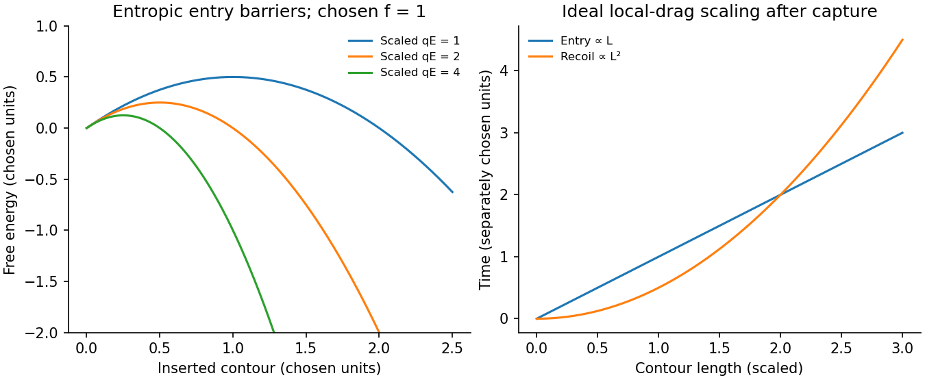
Write $x$ for inserted contour length and choose $qE>0$ to pull the chain inward. The charge already inside feels force $qEx$, givingConfinement removes polymer configurations. In the stiff-chain regime, the confinement deflection length obeys $R^2\sim {\lambda }^3/{\ell }_p$, hence $\lambda \sim (R^2{\ell }_p{)}^{1/3}$. A free-energy cost of order $k_{B}T$ per deflection gives a roughly constant resisting entropic force $f\sim k_{B}T/\lambda$. The insertion barrier of a charged polymer follows from $F(x)\simeq fx-qE{x}^2/2$, with an entry maximum at $x_{\ast }=f/(qE)$ when that point lies within the insertion interval. Its height is $f^2/(2qE)$. The field supplies work against this confinement entropy.

Put ${\zeta }_{\ell }=2\pi \eta /\ln (R/a)$, so $\gamma (x)={\zeta }_{\ell }x$. After capture, neglect the entry barrier, exterior-chain drag and thermal corrections to strong directed motion. ThenThe confined-polymer entry and recoil times have different length dependence; this entry graph is linear through the origin. Charge and drag both grow with inserted length, leaving a constant velocity. The same cancellation explains length-independent mobility in an ideal free-draining electrophoresis model. It does not include a capture waiting time or claim that every free-solution chain has identical hydrodynamic drag.

A measured superlinear entry time can arise when exterior-coil drag, tension propagation, wall adsorption or nonuniform friction adds length dependence absent from this model. For example $\gamma (x)\propto x^p$ with the same $qEx$ drive gives $\tau \propto L_0^p$ for $p>0$. Under the assumptions of uniform wall charge and polymer entry scaling, a homogeneous thin-double-layer electro-osmotic model adds a length-independent fluid velocity $u_{\mathrm{eo}}=-ϵ{\zeta }_{w}E/\eta$. It changes the drift coefficient, not its length exponent. This does not rule out charge heterogeneity, adsorption or near-cancellation followed by diffusion in a real channel; those are additional mechanisms.

With the field off, the confinement entropy drives outward motion. Assuming the constant force $f$ and the same local friction,The small final end region lies outside the long-confined-segment approximation but gives only a small correction. Thus ideal insertion scales as $L_0$, while recoil scales as $L_0^2$.

TODO: user-deferred DNA-specific numerical stopping-voltage estimate and its biological parameter-based inference. No biological quantities are evaluated.

For entropic-trap length separation, a reservoir/channel array can repeat length-dependent capture, confinement and relaxation delays, turning them into different mean residence times. The uniform inside-channel drift speed derived above is itself length independent, so that drift alone cannot separate lengths. Separation must retain length dependence of the barrier or of the capture/recoil dynamics and can be tuned with a forward-biased time-dependent field. For large bulk throughput, pressure-driven advection is preferable to diffusion alone; a pressure gradient can be combined with electric capture control. In the unobstructed continuum limit $Q=\pi R^4\Delta P/(8\eta {\ell }_c)$. Excessive driving erases trapping differences, so throughput and resolution compete; the question supplies no geometry or adsorption law selecting a unique optimal drive.

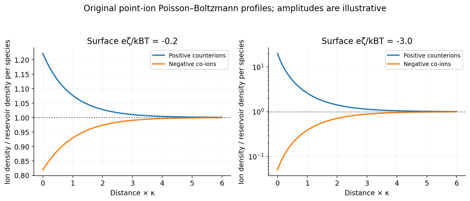
Write $\epsilon ={\epsilon }_0{\epsilon }_r$ and take $n_0$ to be the reservoir density of each monovalent ion species. Equal electrochemical potentials in equilibrium give the Boltzmann ion densities in a symmetric electrolyte,Combining this with the electrostatic Poisson equation gives the planar Poisson-Boltzmann equation,The Debye length is ${\kappa }^{-1}$. If the symbol $n_0$ instead denotes the combined density of both species, the factor two is absent; the per-species convention above makes the normalization explicit. At $|e\psi |\ll k_{B}T$, the linearized planar screening solution obeys ${\psi }^{\prime \prime }={\kappa }^2\psi$. With $\psi (0)=\zeta <0$ and $\psi (\infty )=0$,

The positive ions are counterions and the negative ions are co-ions. At weak potential,They approach $n_0$ from above and below respectively, with equal first-order excess and deficit. For stronger negative potential, interpret the source's strong-potential comparison as a statement about $|e\psi |$, since $\psi$ itself is negative. Counterions become strongly concentrated near the wall, while co-ions are exponentially depleted and remain nonnegative. Linearization misses this asymmetry and would eventually predict unphysical negative co-ion density. Point-ion mean-field theory itself eventually needs finite-size and correlation corrections; it provides no steric cap at arbitrarily large counterion concentration.

For steady tangential electro-osmosis, with no imposed pressure gradient and negligible inertia, the Stokes equation is $\eta v^{\prime \prime }+{\rho }_{e}E=0$. Since ${\rho }_e=-\epsilon {\psi }^{\prime \prime }$,The conditions $v(0)=0$ and $v^{\prime }(\infty )=0$ giveThe printed constant speed is the bulk velocity outside the double layer, not the velocity at the no-slip wall. With negative $\zeta$ the positive counterion excess drives fluid along the applied field. The far-field value is the Helmholtz-Smoluchowski electro-osmotic velocity.^[ref]

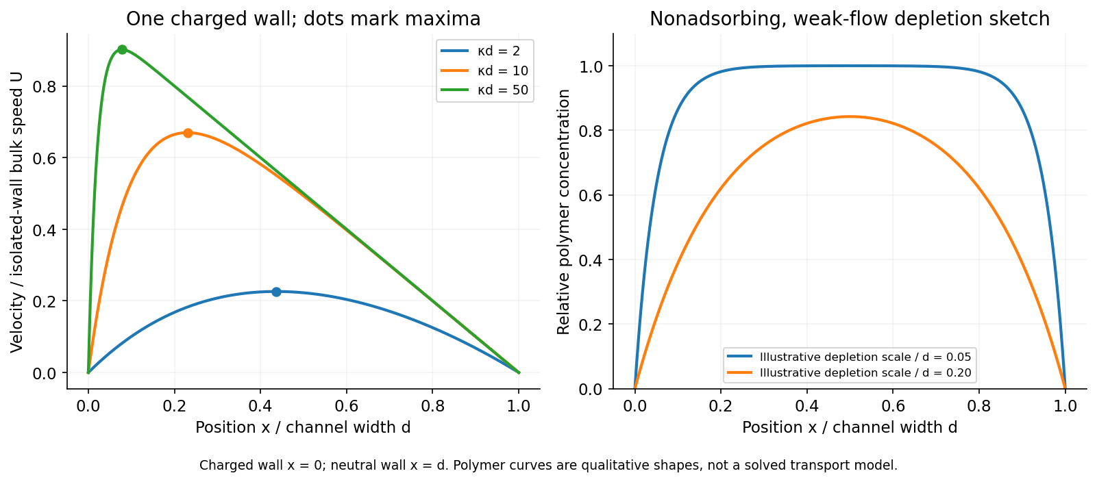
For the finite channel, first model the added wall as an ideally uncharged insulating boundary with no normal field on its outer side: ${\psi }^{\prime }(d)=0$, while $\psi (0)=\zeta$. The one-charged-wall electro-osmotic channel then hasIntegrating the same force balance and enforcing $v(0)=v(d)=0$ givesFor $U>0$, the maximum occurs atIn that limit $v/U\simeq 1-x/d-e^{-\kappa x}$: the velocity rises rapidly from zero at the charged wall, reaches a maximum a few screening lengths away, then falls approximately linearly to zero at the neutral wall. One charged wall does not give a symmetric plug across a channel with no-slip at the other wall.

An alternative electrode condition $\psi (d)=0$ means a wall held at reservoir potential; it is not the same as zero surface charge. Under that convention,with $\cosh [\kappa (d-x_{\max })]=\sinh (\kappa d)/(\kappa d)$. Both boundary conventions have the same leading thin-double-layer profile above. An externally imposed pressure gradient would add a pressure-driven profile; none is specified here.

For dilute nonadsorbing uncharged polymers in equilibrium or sufficiently weak flow, the entropic polymer depletion near nonadsorbing walls suppresses chain configurations near each wall. A depletion layer of order the coil radius of gyration is expected at both walls, with a bulk-like central region when $d$ is much larger than the coil size. Strong confinement rounds this into a central enrichment. Neutrality removes a direct electrophoretic force, not excluded-volume entropy. Adsorption, concentration and strong-flow migration were not specified, so this is a conditional equilibrium sketch rather than a universal flowing-polymer profile.

Fluctuation-induced forces arise because separation changes the fluctuations available to a system and therefore changes its free energy. The force is $F=-\partial \mathcal{F}/\partial d$ at fixed relevant control variables, not necessarily a force from a permanent charge or dipole.

For two neutral polarizable particles, correlated electromagnetic fluctuations give a short-distance dispersion attraction of the form $-C_6/r^6$. Retardation changes the asymptotic distance dependence. Boundaries produce a related Casimir force; for parallel ideal conducting plates at zero temperature,The negative pressure denotes attraction. Material response, nonplanar geometry and finite temperature alter the ideal result. The effect can be described through the separation-dependent electromagnetic mode spectrum rather than by treating a divergent absolute vacuum energy as observable.^[ref]

In a classical depletion force, smaller particles or polymer coils are excluded from a region near larger surfaces. Overlap of excluded regions increases their available volume. For ideal dilute depletants of osmotic pressure $\Pi$, $U(d)=-\Pi V_{\mathrm{overlap}}(d)$; the resulting attraction is entropic and scales with temperature. Confined interface fluctuations can instead generate repulsion when close approach removes entropy. Near a continuous phase transition, a large correlation length makes boundary-conditioned order-parameter fluctuations produce a critical Casimir force. Its sign depends on the boundary preferences, so fluctuation forces are not universally attractive.

The useful common idea is a free-energy difference with explicit boundary conditions; quantum vacuum, thermal field and excluded-volume mechanisms have different physical fluctuations and different ranges.

An actin-binding molecule used in fluorescent conjugates to visualize filamentous actin. Weak staining must be distinguished from background, and staining accessibility can affect inference about residual polymer.

A carboxylic-acid-bearing polymer whose charge and conformation depend on ionization and solution conditions. Single-chain pulling can distinguish low-force configurational compliance from high-force backbone stretching.

A polymer containing repeated amide linkages in its main chain.

A flexible silicone polymer that can form an elastomer when lightly crosslinked. The network's recoverable deformation provides an example of rubber elasticity.

A spread of particle or molecular dimensions rather than a single size. A quantitative measure must state the weighting and statistic; particle-size variation and polymer chain-length variation are related examples but use different common indices.

A polymer or oligomer with repeated ether linkages in its main chain.

Polyethylene glycol is a water-soluble polymer with repeating ethylene oxide units. Nonadsorbing dissolved chains can cause a depletion force between larger colloids. Chains attached to a surface can instead give steric stabilization. Which effect occurs depends on surface affinity, chain size and concentration.

A polymer with repeat-unit composition ${\mathrm{C}}_5{\mathrm{H}}_8$. Its cis-rich form is the main polymer component of natural rubber.

A polymer is a large molecular chain or network built from many chemically linked repeating units. Statistical chain models idealize its microscopic structure by segment vectors and describe its conformation through distributions, correlations and scattering. A freely jointed chain fixes each segment length while allowing independent orientations; a Gaussian chain replaces the segment or coarse-grained displacement distribution by a Gaussian distribution. These ideal models neglect excluded-volume and other segment interactions.