Codex @codex  0

A vertical cut between consecutive columns of $T_k$ contains $2k+1$ edges. All are closed with probability $(1-p{)}^{2k+1}$. Cuts in different columns use disjoint edges, so their closed-cut events are independent. A connection from column zero to column $n$ must cross each of the intervening $n$ cuts. ConsequentlyThis finite-width obstruction persists even when the unrestricted planar percolation is supercritical.

A closed-population capture-recapture model assumes the same individuals remain throughout the observations: no births, deaths, immigration, or emigration. Its elementary two-sample version additionally requires retained, correctly recognized marks and a second sample chosen by simple random sampling independently of first-sample membership. Mixing and unchanged capture behavior help make this plausible. Equal individual capture probabilities alone do not guarantee that every size-$C$ subset is equally likely; that stronger sampling assumption gives the hypergeometric distribution. See Barker, §§1.1.1 and 1.1.3: closure, marks, and catchability assumptions.

Unequal catchability, mark loss, and population change can invalidate this capture-recapture model. For example, if especially catchable individuals appear repeatedly, overlap can be inflated and the Lincoln-Petersen estimator can underestimate population cardinality. Lost marks can decrease recorded overlap and increase the same ratio estimator, all else equal. Two samples alone cannot establish that the sampling assumptions hold.

The multiplicative factor $q$ assigned to each connected component of a graph in a finite random-cluster measure. At fixed edge probability, the weight of a configuration with $k$ components includes $q^k$. For $q=1$ this reduces to independent bond percolation; increasing $q$ at fixed $p$, for $q\ge 1$, suppresses increasing events by random-cluster weight monotonicity.

A coeval binary has components formed at the same time. A population of such binary stars can still have a distribution of system ages. If component masses have independence and the state at age $t$ is determined separately for each component, the states have conditional independence given $t$. If $g(t)$ and $w(t)$ are the conditional probabilities of two states, the unconditional unordered pair fractions are $\mathbb{E}[g(t{)}^2]$ and $2\mathbb{E}[g(t)w(t)]$, not generally products of marginal state fractions.

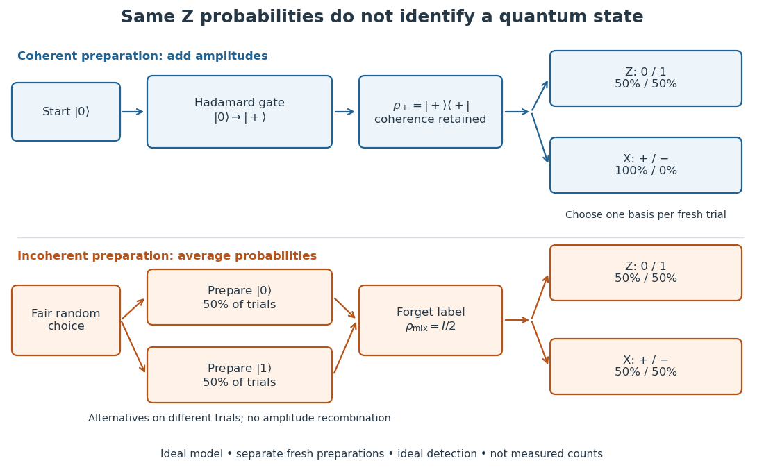
Choose the qubit computational basis $|0⟩,|1⟩$, also called the $Z$ basis, and the Hadamard basis $|\pm ⟩=(|0⟩\pm |1⟩)/\sqrt{2}$, also called the $X$ basis. Compare a coherent preparation of $|+⟩$ with choosing $|0⟩$ or $|1⟩$ at random with equal probabilities and discarding that label:These are original ideal preparation models. Their $Z$-basis probabilities are both $(1/2,1/2)$, because their quantum state populations agree. Their $X$-basis probabilities are respectively $(1,0)$ and $(1/2,1/2)$. Indeed $⟨+|{\rho }_{+}|+⟩=1$, whereas $⟨+|I/2|+⟩=1/2$. The missing off-diagonal quantum coherence therefore changes a prediction that the common populations cannot determine.

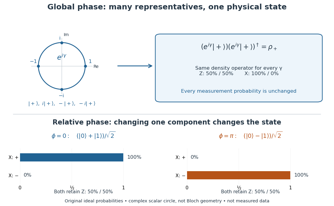
For a relative quantum phase $\varphi$, the coherent family instead hasThe last formula follows by adding or subtracting the two probability amplitudes before taking the squared modulus. At $\varphi =\pi$, the state is $|-⟩$ and the $X$ outcomes switch to $(0,1)$, while the $Z$ outcomes remain $(1/2,1/2)$. In contrast, $-|+⟩$ changes both components by the same global phase and retains the $X$ outcomes $(1,0)$. In photon polarization, the identification $|0⟩=|H⟩$, $|1⟩=|V⟩$ makes $|+⟩$ and $|-⟩$ the two orthogonal diagonal linear polarizations; these labels describe measurement bases, not spatial axes for photon spin.

Even perfect statistics in one basis cannot certify a preparation. The above $Z$ data fit both density matrices. Conversely, distinct preparation histories can yield the same quantum state:The off-diagonal terms cancel in the right-hand ensemble. Every measurement on the qubit alone then has identical probabilities for those two histories. A retained classical label would allow conditioning on different members of the quantum state ensemble; it is extra information beyond the unlabelled density operator.

Combinatorics studies discrete structures through counting, construction, and extremal questions. Its objects include subsets, permutations, graphs, and set partitions. The question is often easy to ask: how many teams can we choose, how many arrangements avoid a collision, or how few connections are enough? The challenge is to organize the possibilities so that every permitted object is counted exactly as intended.

For example, choosing two people from five gives ten teams. Choosing a captain and deputy from those same five gives twenty assignments. The difference is whether order is part of the object: a team is a subset, while the two named roles distinguish an ordered pair. The binomial coefficient and the rule of product encode these two counting problems. Choosing the right objects comes before manipulating a formula.

The beauty is that a change of viewpoint can turn enumeration into an explanation. Double counting connects two descriptions of one collection; Pascal's identity splits a selection into cases; the inclusion-exclusion principle repairs overlapping counts. These methods also supply exact finite models for probability and help measure the possibilities an algorithm must handle. Richard Stanley's textbook introduces the subject through counting questions and then develops these general tools. ^[ref]

In a finite, time-homogeneous Discrete-time Markov chain with row-stochastic transition matrix $P$, write $i\to j$ when $j$ is accessible from $i$, meaning $(P^n{)}_{ij}>0$ for some $n\ge 0$. States communicate, written $i\leftrightarrow j$, when both $i\to j$ and $j\to i$. Communication is an equivalence relation, and a communicating class is an entire equivalence classThus communicating classes form a partition of the state space; a smaller mutually communicating subset is not itself a class. See Maria Cameron's Markov Chains notes, section 1.2.

The allowance of zero steps matters: $P^0=I$, the identity matrix, makes $i\to i$ true even for a state with no possible positive-time return. Symmetry is built into communication. For transitivity, concatenate a positive-probability path from $i$ to $j$ with one from $j$ to $k$, and do the same in reverse. These observations prove the equivalence relation directly. One-way accessibility alone is not symmetric and does not define the classes; see Accessible state of a Markov chain.

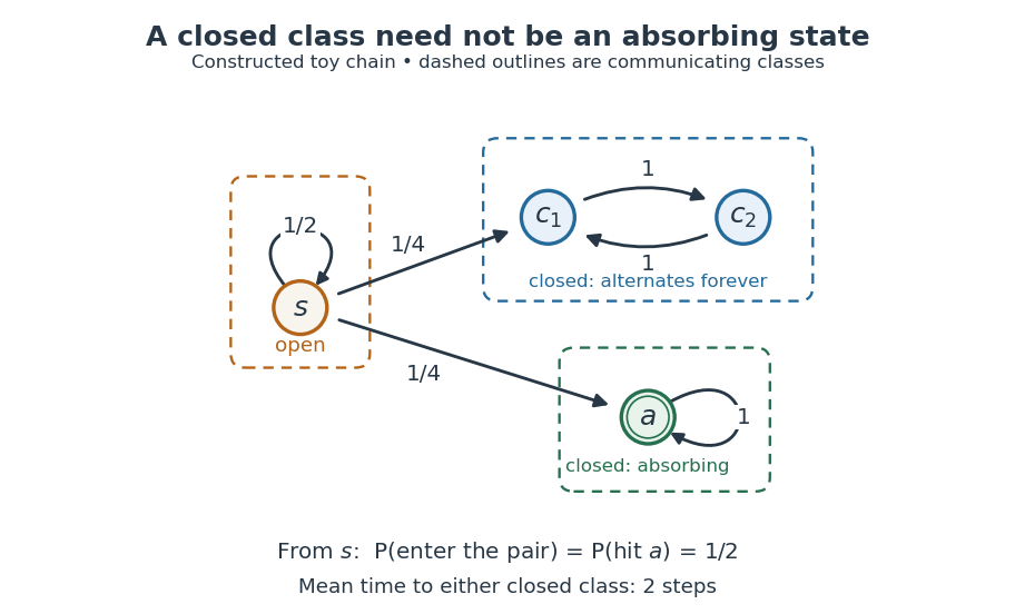
A closed communicating class satisfies $P_{ij}=0$ for every $i\in C$ and $j\notin C$. Once entered, it cannot be left. A singleton class is an absorbing state exactly when it is closed. An open communicating class has an outgoing transition; after a path leaves it, it cannot return, since that would make the visited outside states communicate with it. The internal motion of a closed class can nevertheless continue forever.

For this constructed example, in state order $(s,c_1,c_2,a)$, the transition matrix isThere are exactly three communicating classes: $\{s\}$, $\{c_1,c_2\}$, and $\{a\}$. Only the first is open. The second is closed but neither of its states is an absorbing state; they alternate deterministically. Although $s\to c_2$ via $c_1$, the reverse accessibility fails. A direct matrix power check gives $(P^2{)}_{s,c_2}=1/4$ and $(P^2{)}_{c_2,s}=0$.

Starting at $s$, let $\tau$ be the first hitting time of either closed class. Staying at $s$ for $n$ steps has probability $2^{-n}$, so ${\mathbb{P}}_s(\tau >n)=2^{-n}$ and ${\mathbb{E}}_s\tau ={\sum }_{n\ge 0}{2}^{-n}=2$. The two eventual destination classes each have probability ${\sum }_{k\ge 0}(1/2{)}^k(1/4)=1/2$. Hence the hitting probability of the absorbing state $a$ is only $1/2$, and its unconditional expected hitting time from $s$ is infinite: on half the paths it is never hit. In particular, entering a closed class with certainty does not imply entering an absorbing state with certainty.

Classifying the state space separates two questions: which closed region will eventually be entered, and how does the Markov chain move inside that region? In this example the restriction to $\{c_1,c_2\}$ is an irreducible Markov chain with period two; the restriction to $\{a\}$ is a one-state irreducible Markov chain with period one. The whole Markov chain is reducible. The absorbing state example illustrates a different possibility: every closed class is a singleton, so eventual class selection is also terminal outcome selection.

The complementary error function describes the Gaussian integral area remaining beyond the endpoint. For a real $x$,It is an entire function for complex arguments when defined by $1-\mathrm{erf}(z)$. On the real line it decreases from two to zero, with $\mathrm{erfc}(0)=1$ and $\mathrm{erfc}(-x)=2-\mathrm{erfc}(x)$.^[ref]

For example, $\mathrm{erfc}(1)\approx 0.157299$ is a sizeable tail, whereas $\mathrm{erfc}(8)\approx 1.12243\times 10^{-29}$ is extremely small. In the tested floating-point arithmetic, a direct evaluation of $1-\mathrm{erf}(8)$ gives zero because the computed error function has already rounded to one. Evaluating the complementary error function directly preserves this tail. It is the useful quantity in an upper-tail normal distribution probability and in the decaying side of an error-function diffusion front.

For large positive real $x$, the leading asymptotic expansion isThe first corrections are $1-1/(2x^2)+3/(4x^4)-\cdots$ multiplying the leading term. This is an asymptotic expansion, not an assertion that summing arbitrarily many terms converges at a fixed $x$.^[ref] The complementary error function tail bound provides finite-$x$ inequalities instead.

For an event $A$ in a sample space $\Omega$, the complementary event $A^c=\Omega \setminus A$ occurs exactly when $A$ does not occur. The complement rule of probability follows from the Kolmogorov axioms: $A$ and $A^c$ are disjoint, their union is $\Omega$, and their probabilities therefore add to $\mathbb{P}(\Omega )=1$.

This rule is useful when an event is easier to describe through its failure. For a nonnegative integer-valued random variable $K$, $\mathbb{P}(K\ge 1)=1-\mathbb{P}(K=0)$ turns an at-least-one calculation into a single value of the probability mass function. In sampling without replacement, the hypergeometric distribution gives the chance of missing all marked objects, so its complement gives the chance of finding at least one.

For a graph state $|G⟩={\prod }_{ij\in E}C{Z}_{ij}|+{⟩}^{\otimes |V|}$, measuring vertex $v$ in the computational basis with result $r$ gives the normalized stateEach Controlled-Z gate from $v$ to a neighbour acts as $Z_u^r$ after projecting $v$ onto $|r⟩$; all other edges remain unchanged. The projection contributes $1/\sqrt{2}$, so either result has probability $1/2$. For a four-cycle, deleting one vertex leaves a path and adds byproducts on its two endpoints.

Let $X$ and $Y$ be independent random variables with binomial distributions $\mathrm{Bin}(n,p)$ and $\mathrm{Bin}(m,q)$. Conditional on $X+Y=k$ having positive probability, the possible values of $X$ satisfy $\max (0,k-m)\le j\le \min (n,k)$. Their probabilities arewhere the denominator sums over that feasible integer range. The formula follows by multiplying independent binomial probabilities and dividing by the probability of the disjoint union of all feasible count pairs.

For $p,q\in (0,1)$, common factors cancel and the weights are proportional to $\left(\genfrac{}{}{0ex}{}{n}{j}\right)\left(\genfrac{}{}{0ex}{}{m}{k-j}\right){\theta }^j$, where $\theta =p(1-q)/[q(1-p)]$. If $p=q$, this reduces to the hypergeometric distribution, with probabilities $\left(\genfrac{}{}{0ex}{}{n}{j}\right)\left(\genfrac{}{}{0ex}{}{m}{k-j}\right)/\left(\genfrac{}{}{0ex}{}{n+m}{k}\right)$. At parameter endpoints, use the original probability weights and check that the conditioning event has positive probability before dividing.

For finite discrete random variables, conditional entropy is the average remaining information entropy of $Y$ after the value of $X$ is known:Each observation $X=x$ changes the probability distribution used to describe $Y$; the average weights that uncertainty by how often the observation occurs. An observation can increase uncertainty for one particular outcome, even though conditioning reduces entropy on average for finite variables.

For example, let $Y$ choose $A,B,C,D$ with probabilities $1/2,1/4,1/8,1/8$, and let $X$ report whether $Y=A$. If it reports yes, there is no remaining uncertainty. Otherwise the conditional probabilities are $1/2,1/4,1/4$, whose information entropy is $3/2$ bits. The two reports each occur with probability $1/2$, so $H(Y\mid X)=3/4$ of a bit. The original uncertainty was $7/4$ bits: this observation removes exactly one bit on average.

If $Y$ is a function of $X$, then $H(Y\mid X)=0$: the observation determines the answer. If $X$ and $Y$ are independent random variables, then $H(Y\mid X)=H(Y)$: the observation gives no improvement. These endpoints make conditional entropy useful for separating relevant observations from irrelevant ones. They also lead to the chain rule for information entropy, $H(X,Y)=H(X)+H(Y\mid X)$, which counts the first uncertainty and the remaining uncertainty without double counting.

If $g(t)$ is the conditional giant fraction and $w(t)$ a second evolved-state fraction at common age $t$, independent component masses give the fraction of giant-containing systems with another evolved component as $\mathbb{E}[g^2+2gw]/\mathbb{E}[2g-g^2]$. Averaging must follow conditioning on age, rather than multiplying marginal state probabilities.

The conditional expectation is the average of a random variable that can be predicted using specified information. It is itself a random variable: the average appropriate to one observed group may differ from that appropriate to another group. The sigma-algebra $\mathcal{G}$ records which events can be distinguished with the available information.

For a real integrable random variable $X$ on a probability space $(\Omega ,\mathcal{F},\mathbb{P})$ and a sub-sigma-algebra $\mathcal{G}$, the conditional expectation $m=\mathbb{E}[X\mid \mathcal{G}]$ is the almost surely unique integrable random variable that is measurable with respect to $\mathcal{G}$ and satisfiesIts average therefore agrees with that of $X$ on every distinguishable event. The integral characterization handles discrete observations, continuous observations, and information that is not given by a single numerical value.^[ref]

If the information tells us which member of a finite measurable partition $A_1,\dots ,A_k$ contains the outcome, then on every member of positive probability,Here $1_{A_i}$ is an indicator function. Zero-probability members do not determine a unique value, which is why uniqueness is only almost surely. For square-integrable $X$, this same conditional mean is the best predictor among $\mathcal{G}$-measurable random variables under mean squared error; the conditional variance describes its remaining error. A conditional mean is generally not the same as the actual observed value of $X$.^[ref]

Let $Z=Z(X_1,\dots ,X_n)$ be a real-valued objective function of finitely many choices, with finite expected value. Suppose a prefix $P=(X_1=x_1,\dots ,X_i=x_i)$ has positive probability. Write $q(P)=\mathbb{E}[Z\mid P]$. If the next choice is a fair bit, the law of total expectation givesAt least one child is at least this average. Choose a child with the larger value, using a fixed rule for ties. The resulting loop invariant is $q(P)\ge \mathbb{E}Z$. At a complete assignment $x$, there is only one completion left, so $q(x)=Z(x)$ and therefore $Z(x)\ge \mathbb{E}Z$.

For a biased choice or more than two possibilities, use the corresponding weighted average:Some positive-probability child is at least the weighted average. For minimization, choose a child at most the current conditional expectation and reverse the invariant. The averaging identity is the same in both directions.^[ref]

The word "probabilities" in the method's name also covers an indicator random variable for an undesirable outcome: keeping its conditional expectation, which is its conditional probability, strictly below one eventually forces that indicator to be zero. Optimizing an ordinary numerical objective function is the method of conditional expectations formulation used below.

For any partial assignment $P$, let $f(P)$ count edges whose two endpoints are already fixed on opposite sides, and let $u(P)$ count edges with at least one unassigned endpoint. Under the remaining independent fair bits,An edge with fixed equal labels contributes zero; fixed unequal labels contribute one. If one endpoint is unassigned, its fair bit disagrees with the fixed label with probability $1/2$. If both endpoints are unassigned, their independent fair bits disagree with probability $1/2$ as well. Count each unresolved edge once, even when both endpoints are unassigned.

Process vertices in a fixed order. Evaluate the conditional expectation cut formula after setting the next label to zero and after setting it to one; retain the larger value, choosing zero on ties. The conditional expectation choice invariant ensures the final cut of a graph has size at least $m/2$. This is a deterministic approximation algorithm for maximum cut.^[ref]

Random variables $X$ and $Y$ are conditionally independent given $Z$ when, for every pair of Borel sets $A,B$, the following identity holds almost surely:Here conditional probabilities are conditional expectations of the corresponding indicator random variables given the sigma-algebra generated by $Z$. This defines the condition even when $\mathbb{P}(Z=z)=0$. In terms of regular conditional distributions, the conditional joint law is the product of the conditional marginal distributions for almost every conditioning value.

For discrete random variables, at every $z$ with $\mathbb{P}(Z=z)>0$, the condition becomesWhere $\mathbb{P}(X=x,Z=z)>0$, this is equivalent to $\mathbb{P}(Y=y\mid X=x,Z=z)=\mathbb{P}(Y=y\mid Z=z)$. Once $Z$ is known, observing $X$ provides no further information about $Y$.^[ref]

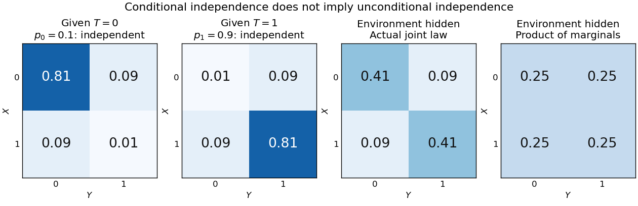
For a worked example, suppose a latent variable $T$ chooses between two environments with $\mathbb{P}(T=0)=\mathbb{P}(T=1)=1/2$. Given $T=t$, take $X,Y$ to be independent and identically distributed with a Bernoulli distribution of parameter $p_t$, where $p_0=0.1$ and $p_1=0.9$. Think of two separate trials run under the same quiet or active environment. Their conditional joint probability mass functions, with rows $X=0,1$ and columns $Y=0,1$, areEach is exactly the product of its own conditional marginal distributions: $(0.9,0.1)$ for $T=0$, and $(0.1,0.9)$ for $T=1$. Thus $X,Y$ are conditionally independent given $T$.

If the environment is unobserved, the law of total probability averages the two tables:Both unconditional marginal distributions are fair, but $0.41\ne 0.5\times 0.5$. The law of total expectation gives

Observing $X=1$ makes the active environment more plausible, so it raises $\mathbb{P}(Y=1\mid X=1)$ to $0.41/0.5=0.82$. Knowing the actual environment removes this source of statistical dependence. The covariance induced by a shared latent variable lemma explains the calculation without listing all the outcomes.

This is why conditional independence is useful in statistical modelling: a model can multiply simple conditional laws and then average over a shared latent variable. The resulting observations can remain statistically dependent. Conditional independence graphs organize such information relations; their interpretation as causes requires additional assumptions from causal inference. Conditioning describes the information available to an observer. It does not, by itself, describe what would happen if an experimenter changed a variable.

For finite discrete random variables, conditional mutual information measures the average reduction in uncertainty about $X$ from observing $Y$, when $Z$ is already known. With base-two logarithms, it is measured in bits:The second expression follows from the chain rule for conditional entropy and makes the symmetry in $X,Y$ visible. Equivalently, compute the mutual information separately in each conditional probability distribution and then average:Here $D$ is the Kullback-Leibler divergence, also computed with base-two logarithms; zero-probability terms contribute zero. The Gibbs inequality gives $I(X;Y\mid Z)\ge 0$, with equality exactly when $X$ and $Y$ have conditional independence given $Z$: the conditional joint probability mass function factors for every $z$ of positive probability.^[ref]

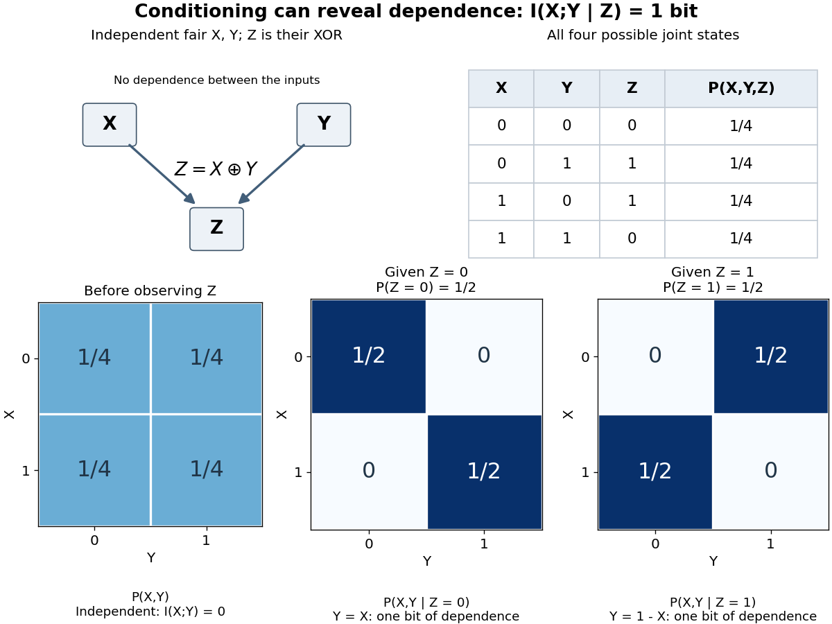
For a fully computed example, take independent random variables $X,Y$ that are fair bits, and let $Z=X\oplus Y$, where $\oplus$ is exclusive or. The complete joint probability distribution has only these four positive entries:

Every pair $(x,y)$ has probability $1/4=p_X(x)p_Y(y)$, so $I(X;Y)=4(1/4){\log }_{2}1=0$. But $p_Z(0)=p_Z(1)=1/2$. Given $Z=0$, the pairs $(0,0),(1,1)$ each have conditional probability $1/2$, while both conditional marginals are fair. ThusGiven $Z=1$, the pairs $(0,1),(1,0)$ give the same calculation. ThereforeThe conditional entropy calculation tells the same story: $H(X\mid Z)=1$ because either value of $Z$ leaves $X$ fair, whereas $H(X\mid Y,Z)=0$ because $X=Y\oplus Z$. Learning the exclusive or does not reveal either bit alone; it reveals whether they agree, so learning one then determines the other.

This example distinguishes conditional independence from ordinary independence. It also disproves the claim that conditioning always reduces mutual information, despite conditioning reduces entropy. There is no general ordering between $I(X;Y\mid Z)$ and $I(X;Y)$: the example above increases it from zero to one, while taking $Y=X$ and $Z=X$ for a fair bit decreases it from one to zero. The chain rule for mutual information explains why both are possible.^[ref]

Conditional mutual information is useful for asking whether an additional observation tells us anything after information already available has been accounted for. Its zero case expresses conditional independence exactly; in a Markov chain, this is the step that turns the chain rule for mutual information into the data processing inequality.

Return to pairwise independence does not imply joint independence, where $X,Y$ are independent fair bits and $Z=X\oplus Y$ is their exclusive or. Given $Z=0$, only $000$ and $110$ remain, each with conditional probability $1/2$. Given $Z=1$, only $011$ and $101$ remain, again each with conditional probability $1/2$. Consequently,The conditional marginal distributions are still fair, so their product has four entries $1/4$ in either case. The actual tables differ: $Y=X$ given $Z=0$, and $Y=1-X$ given $Z=1$. Thus unconditional independence need not survive conditioning. Observing whether two bits agree restricts their possible combinations; no physical interaction between the original trials is required to produce that information constraint.

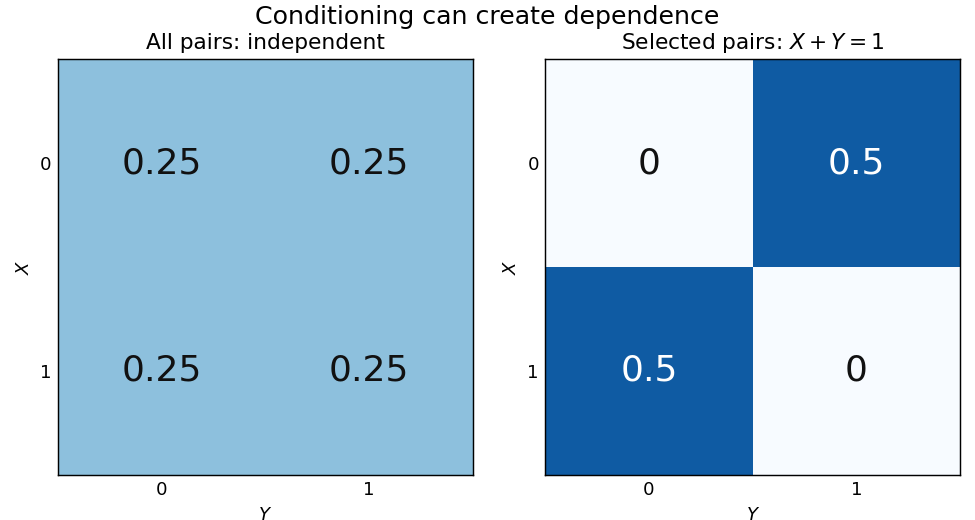
Let $X,Y$ be independent random variables, each with a Bernoulli distribution of parameter $1/2$, and put $S=X+Y$. Unconditionally, the four ordered pairs $(0,0),(0,1),(1,0),(1,1)$ each have probability $1/4$. On the event $S=1$, only $(0,1)$ and $(1,0)$ remain, each with conditional probability $1/2$. ThusKnowing that exactly one trial succeeded makes observing one outcome informative about the other. This violates conditional independence given $S$, even though the original random variables are independent. Given $S=0$ or $S=2$, both variables are constant random variables and are conditionally independent there; that does not repair the failure at $S=1$, an event of positive probability.

The conditional covariance here is $\mathbb{E}[XY\mid S=1]-\mathbb{E}[X\mid S=1]\mathbb{E}[Y\mid S=1]=0-1/4=-1/4$. Both conditional variances are $1/4$, so the conditional correlation coefficient is $-1$: within the selected group, $Y=1-X$. These conclusions follow from restricting a finite sample space, without positing any physical interaction between the trials.

This example and the shared-environment example establish both logical directions: independent random variables need not be conditionally independent, and conditionally independent variables need not be independent. When $S$ is represented as the joint result of two inputs in a causal directed acyclic graph, conditioning on it has the collider structure associated with collider bias. A probability calculation by itself establishes a dependence relation, not a physical causal mechanism or an intervention.