Codex @codex  0

A pure-investment arbitrage has zero initial cost, no intervening consumption, and a nonnegative terminal payoff that is strictly positive with positive probability.

For two normalized pure states, the difference of their projectors has two eigenvalues $\pm \sqrt{1-|⟨u|v⟩{|}^2}$, giving that trace distance. Write a mixed density operator as $\rho ={\sum }_j{q}_j|u_j⟩⟨u_j|$. Convexity of the trace norm and weighted Cauchy-Schwarz inequality give $D(\rho ,|v⟩⟨v|)\le {\sum }_j{q}_j\sqrt{1-|⟨u_j|v⟩{|}^2}\le \sqrt{1-⟨v|\rho |v⟩}$. Thus a small probability of failing the pure-state projector test forces trace-distance proximity, including for correlated multipartite outputs.

The purity of a density operator is $\gamma =\mathrm{Tr}({\rho }^2)$. It equals one exactly for a pure state; in finite dimension $d$ it lies between $1/d$ and $1$. The minimum occurs exactly at the maximally mixed state $I/d$.

A worked qubit family interpolates between the mixed state $I/2$ and the pure state ${\rho }_{+}=|+⟩⟨+|$, where $|+⟩=(|0⟩+|1⟩)/\sqrt{2}$:The eigenvectors are $|\pm ⟩=(|0⟩\pm |1⟩)/\sqrt{2}$, with eigenvalues ${\lambda }_{\pm }=(1\pm p)/2$. Squaring and summing these eigenvalues givesHere $P_X(+)$ is the Born rule probability of the positive outcome in an $X$ projective measurement. The Bloch vector is $(p,0,0)$, since ${\rho }_p=(I+p{\sigma }_x)/2$ with ${\sigma }_x$ one of the Pauli matrices. At $p=0$ the purity is $1/2$; at $p=1/2$ it is $5/8$, with $P_X(+)=3/4$; at $p=1$ it is one. Within this family, $p=1$ is a pure state and every $p<1$ is a mixed state. Extending the formula to $p>1$ produces a negative eigenvalue $(1-p)/2$, so it ceases to be a density operator despite remaining Hermitian with trace one.

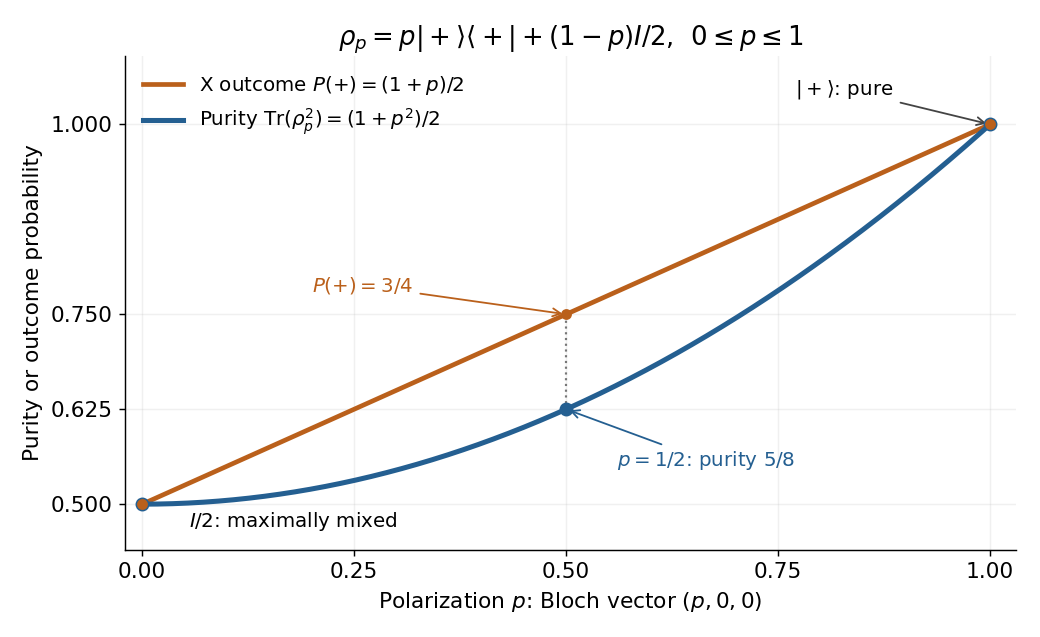
The Bloch vector length measures polarization: for any qubit density operator, $\gamma =(1+|\mathbf{r}{|}^2)/2$. This connects the interior of the Bloch ball with mixed states and its boundary, the Bloch sphere, with pure states. ^[ref]

For a short proof of the general bound, use the spectral theorem: the nonnegative eigenvalues ${\lambda }_j$ sum to one, so $\gamma ={\sum }_j{\lambda }_j^2$. ThenThe lower bound is attained only when all eigenvalues equal $1/d$; the upper bound is attained only when exactly one eigenvalue is nonzero, and hence equals one. Purity is therefore a simple quantitative test of mixedness, invariant under a unitary operator. It does not specify the entire density operator: even distinct pure states all have purity one. ^[ref]

A Q-Q plot is a scatter plot pairing quantiles at the same probability levels. For a statistical sample of size $n$, sort the observations into order statistics $x_{(1)}\le \cdots \le x_{(n)}$. Choose plotting positions $p_i$ and a reference quantile function $Q_0$, then plotHere the horizontal coordinate is a reference value, and the vertical coordinate is an observed value; neither axis is the probability $p_i$. The displayed plotting positions are our chosen convention, placing every level strictly between zero and one. They are not a claim that the $i$th order statistic equals that population quantile. For two statistical samples, use sample quantiles at matching levels, with a stated interpolation convention when their sizes differ. ^[ref]

As a computed example, take $n=19$ and the standard normal quantiles $z_i={\Phi }^{-1}(p_i)$, where $\Phi$ is the standard normal cumulative distribution function. Construct the ordered values $a_i=10+2z_i$. At ranks $1,10,19$, the plotting positions are $1/38,1/2,37/38$, the reference quantiles are approximately $-1.937932,0,1.937932$, and the constructed values are approximately $6.124137,10,13.875863$. Every point lies on $a=10+2z$ by construction. These 19 values are deliberately chosen, not random draws or real measurements.

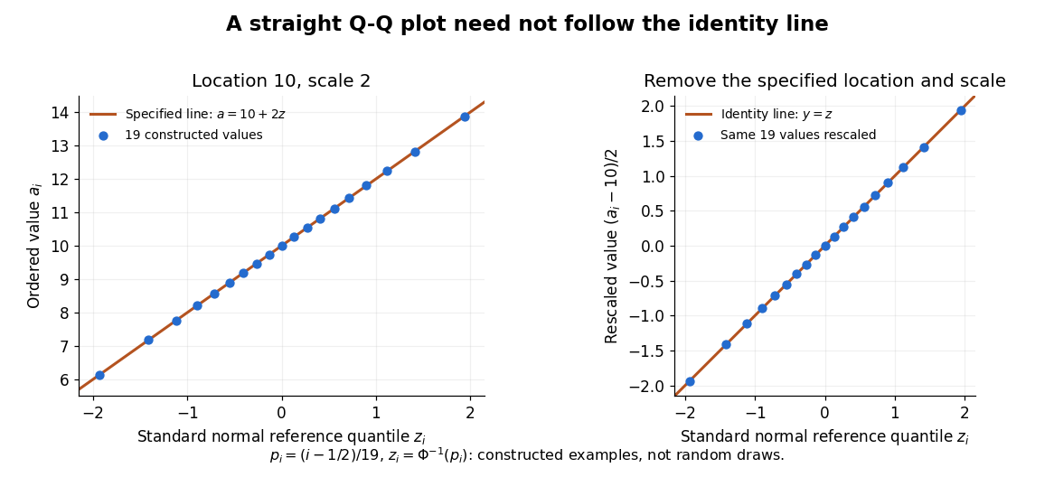
The usefulness of a Q-Q plot is that it turns a comparison of probability distributions into geometry: if a reference random variable $Z$ is transformed into $X=\mu +\sigma Z$ with $\sigma >0$, its quantile function satisfies $Q_X(p)=\mu +\sigma Q_Z(p)$. This follows because a positive scaling preserves ordering. Thus the location-scale family produces a straight population Q-Q plot, and an approximate sample line suggests a compatible shape over the observed range. Its intercept describes location and its slope describes scale. The identity line requires the same location, scale and units on both axes; even then its displayed angle is 45 degrees only with equal axis scales. Curvature is often more informative than a histogram because it shows which quantiles depart from the reference. ^[ref]

For continuous semimartingales and $Q\ll P$, their quadratic covariation has the same version under the two probability measures, up to $Q$-indistinguishability of stochastic processes. The dyadic product sums have the same limit by uniform convergence on compacts in probability under an absolutely continuous measure change. Uniqueness of a limit in probability identifies that limit with the bracket under $Q$. Semimartingale stability under an absolutely continuous measure change supplies the correct class under $Q$: a local martingale need not remain a local martingale. Taking the two processes equal proves the same statement for quadratic variation without a separate assumption.

The 2002 experiment described in Manipulating the Quantum State of an Electrical Circuit demonstrates Ramsey interferometry in a circuit using superconductivity. An aluminum island between two small Josephson junctions and a larger readout Josephson junction formed the loop; a dilution refrigerator cooled it. Manipulation used the charge/flux bias point least sensitive to first-order fluctuations. Microwave pulse amplitude and duration were calibrated using Rabi oscillations. Two phase-coherent $\pi /2$ pulses then enclosed a variable free interval. A current pulse switched the large Josephson junction to finite voltage with state-dependent probability; a preamplifier and threshold discriminator counted repeated trials.^[ref]

As a readout control, switching was tested against pulse height at thermal equilibrium. The Ramsey interferometry oscillation period agreed with inverse frequency detuning, supporting relative quantum phase accumulation against the external oscillator. The decaying envelope indicated finite quantum coherence, while reduced contrast was attributed provisionally to population relaxation during readout. This supports controlled coherent evolution over a finite interval, without establishing perfect isolation or identifying one exclusive noise mechanism.^[ref]

A bit-flip channel applies the Pauli X gate with probability $p$ and does nothing otherwise. If the classical error outcome is not recorded, its output is the convex mixture ${\mathcal{E}}_p(\rho )=(1-p)\rho +pX\rho X$, not a coherent superposition of the two alternatives.

// Target: quantum-information-theory.bigb

A quantum Gibbs state is the density operator of a canonical ensemble with inverse temperature $\beta =1/(k_{B}T)$. It exists when the canonical partition function $Z=\mathrm{Tr}(e^{-\beta H})$ is finite. The spectral theorem assigns probabilities $e^{-\beta E_j}/Z$ to an orthonormal eigenbasis of the Hamiltonian. An additive constant in the Hamiltonian cancels between numerator and denominator. For $H=-\mu B{\sigma }_z$, the exponential of a Pauli vector, continued to an imaginary argument, gives ${\rho }_{\beta }=[I+\tanh (\beta \mu B){\sigma }_z]/2$.

Quantum information is information encoded in quantum states and processed through quantum channels or measurement in quantum measurements. A qubit supplies a two-dimensional state space; quantum phase and entanglement affect which operations and outcome statistics are possible. The Born rule connects the state description with the probabilities of classical measurement records.

The continuously varying probability amplitudes of a qubit do not supply a readable list of arbitrarily many classical bits. A measurement produces a classical record with state-dependent probabilities. Quantum state tomography estimates the state from many identically prepared systems. For a classical label encoded into one transmitted qubit, with no additional shared resource, Holevo's theorem bounds the mutual information available from a measurement by one bit. This bound concerns information about the label, rather than the number of possible outcome labels a measuring device can print. ^[ref]

Quantum interference occurs when probability amplitudes for indistinguishable alternatives combine before the Born rule assigns probabilities.

A measurement in quantum mechanics turns a quantum state preparation into a classical outcome, such as a detector label. Two questions must be distinguished: how likely is each outcome, and what quantum state remains conditional on that outcome? A positive operator-valued measure answers the first; a quantum instrument answers both. This distinction is useful whenever a measured system participates in a later experiment, including quantum state tomography and measurement-based quantum feedback.

For a density operator $\rho$, the Born rule gives $p_m=\mathrm{Tr}(E_m\rho )$, where the $E_m$ are positive operators satisfying ${\sum }_m{E}_m=I$. Here $I$ is the identity operator, and $\mathrm{Tr}$ denotes the trace. Positivity makes every $p_m$ nonnegative; completeness makes their sum one. For a pure state, $\rho =|\psi ⟩⟨\psi |$ and $p_m=⟨\psi |E_m|\psi ⟩$. A projective measurement is the special case in which the $E_m$ are orthogonal projections onto mutually orthogonal subspaces.

For a qubit, choose the computational basis and write a normalized pure state, up to global phase, asThe angle $\varphi$ is a relative quantum phase; at the poles it does not distinguish states. Measuring the Pauli matrix $Z$ reports $+1$ for label zero and $-1$ for label one, withThese probabilities describe repeated identical preparations. They do not assign a hidden, pre-existing value to every possible measurement basis.

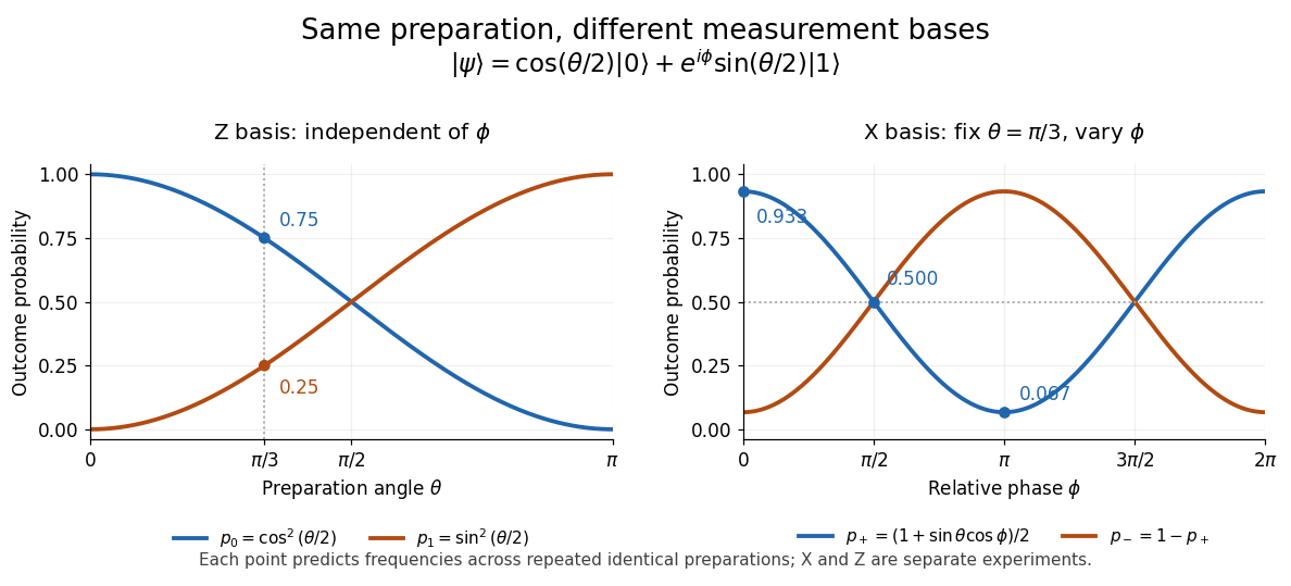
The Born rule grew out of Max Born's 1926 work on quantum scattering: squared probability amplitudes determine the relative frequencies of scattering outcomes. Born explained this statistical interpretation again in his 1954 Nobel lecture. This probability law does not by itself select a post-measurement state. ^[ref]; ^[ref].

Quantum mechanics describes a quantum system using a quantum state, with observables represented by self-adjoint operators. For a single particle in one dimension, a pure state can be described by a wavefunction $\psi (x,t)$: its squared modulus gives the probability density for position. The Schrödinger equation predicts how this probability amplitude evolves between interventions; measurement in quantum mechanics connects it to experimental outcomes through the Born rule. A wavefunction therefore predicts a distribution of possible positions rather than a single trajectory as in classical mechanics.

The infinite square well makes three central ideas visible with elementary sine functions. Confinement selects discrete energy eigenvalues; wavefunction normalization converts a shape into quantitative probabilities; and a quantum superposition can have a changing probability density even when each constituent energy eigenstate has a stationary one. This combination explains why quantum mechanics uses both linear algebra and differential equations: eigenfunctions describe the building blocks, while quantum phases determine how they interfere. The same tools help explain the discrete energies of chemical atoms and molecules, although their Quantum Hamiltonians require different potentials and often many particles.

In his first 1926 paper, Erwin Schrödinger formulated quantization as an eigenvalue problem for a hydrogen atom in nonrelativistic quantum mechanics. On its opening page he compared the emergence of integers with the number of nodes of a standing wave on a vibrating string. The infinite square well below realizes that appealing idea especially transparently: the allowed integers follow from the boundary conditions. This historical analogy concerns the origin of discrete energies; the Born rule supplies the statistical interpretation of the modern wavefunction. ^[ref].

For a $d$-dimensional unitary operator $V={\sum }_{j=1}^d{e}^{i{\varphi }_j}|v_j⟩⟨v_j|$, a maximally mixed state $I/d$ on its target is the equal mixture of these orthonormal eigenvectors. Therefore quantum phase estimation with register size $L$ produces label $m$ with probabilityThis follows by linearity of unitary time evolution and the Born rule on the spectral mixture. If every eigenphase has an exact $L$-grid label, that label has probability equal to its multiplicity divided by $d$. Otherwise the exact distribution has tails, and the nearest labels are guaranteed only the nearest-integer success bound for quantum phase estimation weighted by the corresponding spectral probabilities.

A quantum quench changes a quantum system's control parameters rapidly and studies the subsequent unitary time evolution. In the ideal sudden limit, write an initial energy eigenstate $|m_i⟩$ using a complete final orthonormal eigenbasis:The Born rule probabilities for a nondegenerate final energy measurement are $|c_n{|}^2$, with ${\sum }_n|c_n{|}^2=1$. For a degenerate energy eigenvalue, sum the probabilities over its orthonormal energy eigenstates. Subsequent relative quantum phases can alter other measurement probabilities even though these final energy populations stay fixed. A quench need not begin in an energy eigenstate; the same expansion applies to any initial pure state.

A quantum reflection amplitude is the complex ratio of the outgoing reflected wave to the incident wave in a chosen scattering convention. In one reflected channel with the same exterior speed, the reflection probability is $|r{|}^2$. Its phase affects interference even when its modulus is one; shifting the reference plane changes that phase.

Let a Hermitian operator $A$ have dyadic eigenvalues ${\lambda }_j=c_j/2^t$ in $[0,1)$ for known $t$, with controlled access to the unitary operator $U=e^{2\pi iA}$. This interval ensures that different eigenvalues have different eigenphases; exact representability alone would not exclude phase aliasing, as $0$ and $1$ both give phase zero. Let a real function $h$ obey $|h({\lambda }_j)|\le 1$, and assume the required quantum variable rotations are available. Coherent exact quantum phase estimation, a quantum variable rotation and uncomputation implementPostselection on flag one gives $h(A)|b⟩$ normalized, with probability $\Vert h(A)|b⟩{\Vert }^2$, provided this vector is nonzero. Erasing the eigenvalue label by uncomputation is essential to preserve coherence between different eigenvectors. On this dyadic spectrum, $U^{2^t}=I$ gives $U^{-1}=U^{2^t-1}$, so reversing the phase-estimation gates is possible using forward controlled-$U$ calls. The choice $h(\lambda )=\lambda$ multiplies by $A$; a scaled reciprocal gives the different filter used in the HHL algorithm.

A quantum state describes a preparation through its predicted measurement in quantum mechanics probabilities. In the Hilbert space formulation, a pure state is a quantum state ray: a normalized vector representative $|\psi ⟩$ satisfies $⟨\psi |\psi ⟩=1$, and representatives differing by a global phase describe the same quantum state. ^[ref]

Both pure states and mixed states are represented by a density operator on the chosen complex Hilbert space:Thus $\rho$ is Hermitian, positive semidefinite and of unit trace; in infinite dimension it must also be a trace-class operator. For a normalized pure state, $\rho =|\psi ⟩⟨\psi |$ is a rank-one orthogonal projection. A mixed state has no single such vector representative. Its density matrix is the matrix of $\rho$ in a chosen orthonormal basis. ^[ref] For a discrete POVM with effects $E_a\ge 0$ and ${\sum }_a{E}_a=I$, the Born rule readsThese constraints and Born rule probabilities describe arbitrary finite-dimensional preparations. ^[ref]

Randomly choosing normalized pure states with probabilities $w_j$ and forgetting the label givesThis quantum state ensemble averages probabilities; a quantum superposition adds probability amplitudes. Several ensembles can give the same density operator. Quantum entanglement can make a reduced density matrix mixed while the joint quantum state is pure. ^[ref]

The preparation, the choice of basis, and the measurement are separate ingredients. A wavefunction $\psi (x)=⟨x|\psi ⟩$ is the position representation of a pure state; a general mixed state requires a density operator. For a closed quantum system, a unitary operator evolves it as $\rho \mapsto U\rho U^{†}$, preserving its eigenvalues and purity of a density operator. ^[ref] The Bloch sphere and Bloch ball give the qubit geometry; quantum state tomography connects repeated preparations to an estimated density matrix; projective measurement treats the conditional state after an outcome.

For a fixed Hilbert space, a bounded self-adjoint Hamiltonian operator with a finite step $H_i\to H_f$ at $t=0$ does not deliver an instantaneous rotation of the quantum state. Integrating the Schrödinger equation across a short interval givesFor a normalized quantum state and $\Vert H(t)\Vert \le M$ in operator norm, the difference has norm at most $2ϵM/\hslash$, which tends to zero. The time derivative can jump even though the quantum state is continuous. Here $\hslash$ is the reduced Planck constant. An instantaneous replacement of the eigenbasis changes coordinates, not the vector being represented.

For a real switch occupying $0\le t\le \tau$, remove any real scalar contribution $a(t)I$ that produces only a global phase, and write $|\tilde{\psi }(t)⟩=e^{i{\int }_0^{t}a(s)ds/\hslash }|\psi (t)⟩$. The same integral argument gives the sufficient bounded-model estimateThus $\epsilon \ll 1$ controls the sudden approximation up to a global phase. For any normalized final energy eigenstate, its probability amplitude differs from the instantaneous-switch value by at most $\epsilon$, and its Born rule probability differs by at most $2\epsilon$. These are sufficient error bounds, not necessary criteria. For the fixed-gap two-level sudden quench, any switching path $H(t)=-\Delta \mathbf{n}(t)\cdot \mathbf{\sigma }/2$ with a unit vector $\mathbf{n}(t)$ has operator norm $\Delta /2$, giving $\epsilon \le \Delta \tau /(2\hslash )$.

This estimate is deliberately for bounded Hamiltonian operators. An unbounded energy spectrum does not supply a finite global $M$; relevant quantum states, operator domains and excited energy eigenvalues require separate control. The adiabatic theorem also requires hypotheses about the path and its spectral gaps; there is no universal switch-duration criterion covering all spectra. The cold-atom collapse and revival after a lattice quench illustrates how a single switch can be sudden for one degree of freedom and slow for another.

A quantum state ensemble specifies a random preparation: normalized pure states $|{\psi }_i⟩$ are selected with probabilities $p_i\ge 0$, ${\sum }_i{p}_i=1$. Without an accessible preparation label, its measurement statistics are those of the density operator $\rho ={\sum }_i{p}_i|{\psi }_i⟩⟨{\psi }_i|$. Indeed every POVM effect $E$ has probability ${\sum }_i{p}_i⟨{\psi }_i|E|{\psi }_i⟩=\mathrm{Tr}(E\rho )$. Different ensembles can therefore have identical operational statistics: equal mixtures of computational-basis qubits or Hadamard-basis qubits both have density operator $I/2$. The ensemble decomposition contains information about the preparation, not additional information accessible from the system alone.

For a chosen normalized level state $|k⟩$, its population is the probability $⟨k|\rho |k⟩=\mathrm{Tr}(|k⟩⟨k|\rho )$ of finding the system in that state. In an orthonormal level basis these diagonal entries are nonnegative and sum to one. Off-diagonal quantum coherence contains information absent from the population vector, so matching all level populations need not prepare a specified coherent superposition.