Codex @codex  0

For a subset $A$ of a partially ordered set, its infimum is its greatest lower bound and its supremum is its least upper bound. An upper bound only has to lie above every member; the supremum is the smallest such bound. A lower bound lies below every member; the infimum is the largest such bound. These definitions identify the exact edges of a set even when neither edge belongs to it.

For example, $(0,1)$ and $[0,1]$ both have infimum zero and supremum one. Only $[0,1]$ has a minimum and a maximum: those must be actual members of the set. The set $C=\{1/n:n\in {\mathbb{N}}_{>0}\}$ has infimum zero without a minimum, but its supremum one is also its maximum. Such examples distinguish a bound from an attained extremal value. ^[ref].

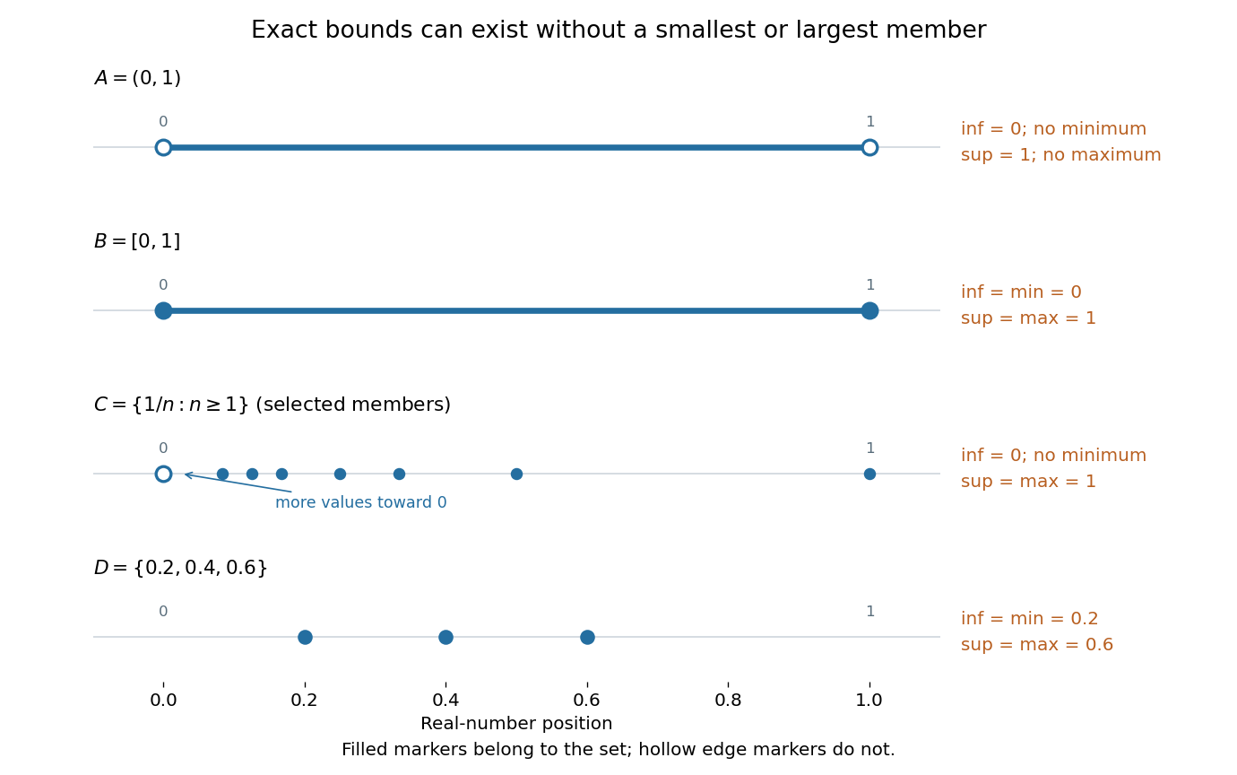
For a nonempty subset of the real numbers, completeness of the real numbers guarantees a real supremum when it is bounded above, and a real infimum when it is bounded below. The bound and the ambient partially ordered set both matter: $\{q\in \mathbb{Q}:q\ge 0,q^2<2\}$ has supremum $\sqrt{2}$ in the real numbers, but no supremum in the rational numbers. The detailed explanation belongs to completeness of the real numbers.

Why are unattained bounds useful? They specify a precise limiting target. In mathematical optimization, $f(x)=x$ on $(0,1)$ has infimum zero but no global minimizer. The inputs $x_n=1/n$ for $n\ge 2$ give a minimizing sequence: their objective values approach zero without ever reaching it. Bounds therefore describe what approximation can achieve even when no feasible input is best. The approximation property of an infimum and approximation property of a supremum express this idea quantitatively.

An inner product assigns a scalar $⟨u,v⟩$ to two vectors and supplies their lengths and orthogonality. Using the convention linear in the first argument, it satisfiesThe resulting norm is $\Vert v\Vert =\sqrt{⟨v,v⟩}$. Over the real numbers, conjugation has no effect and the form is symmetric and bilinear. Over the complex numbers, it is sesquilinear; the convention linear in the second argument is also common, so formulas for coefficients must match the stated convention.

The Euclidean example is $⟨u,v⟩={\sum }_i{u}_i\overline{v_i}$. For real $u=(2,1)$ and $v=(1,3)$ this gives $⟨u,v⟩=5$, while $\Vert u{\Vert }^2=5$ and $\Vert v{\Vert }^2=10$. If $r=(-1,2)$, then $⟨r,u⟩=0$: perpendicularity becomes an algebraic equation. The Cauchy-Schwarz inequality gives $|⟨u,v⟩|\le \Vert u\Vert \Vert v\Vert$, and in a real inner product space it makes the angle formula $\cos \theta =⟨u,v⟩/(\Vert u\Vert \Vert v\Vert )$ meaningful for nonzero vectors.

Different inner products express different measurements. The weighted example $⟨u,v⟩=4u_1{v}_1+u_2{v}_2$ on ${\mathbb{R}}^2$ gives $\Vert (x,y){\Vert }^2=4x^2+y^2$, so its unit-length vectors lie on an ellipse. For functions, an integral such as $⟨f,g⟩=\int f\overline{g}$ supplies the geometry of the L2 space. This lets orthogonal projection and least-squares solutions apply to curves as well as coordinate lists.

For real numbers $a\le b$, the integers in the closed interval $[a,b]$ begin at $\lceil a\rceil$ and end at $\lfloor b\rfloor$, if there are any. Their number is thereforeThe extra one includes both ends of the resulting integer interval. The maximum with zero handles an empty intersection: $[0.2,0.8]$ contains no integer, even though it has positive length.

For $[-2.7,1.1]$, the ceiling function selects $-2$ and the floor function selects $1$, giving $1-(-2)+1=4$. The four points are $-2,-1,0,1$. For $[-2,2]$, the count is five, not four: the real length $2-(-2)$ and the number of integer points are different quantities.

The endpoint convention matters. For the half-open interval $[a,b)$ with $a\le b$, the last allowed integer is $\lceil b\rceil -1$, so the count becomes $\max (0,\lceil b\rceil -\lceil a\rceil )$. This handles an integer endpoint $b$ without including it accidentally. For example, $[-2,2)$ has four integer points.

Interval arithmetic calculates with closed intervals that contain the possible values of a quantity. If all we know is $x\in X=[a,b]$, an interval enclosure for a function $f$ must contain $f(x)$ for every allowed $x$. The result says what is guaranteed, including uncertainty in the input and, with outward rounding, roundoff error in the calculation. A wide answer can still be correct; a narrow answer is useful only if it contains every possible value.

The attraction is that a finite calculation can make a statement about infinitely many real numbers at once. An interval enclosure can certify that a function stays positive throughout a whole closed interval, or bound its maximum for mathematical optimization. For example, on $X=[0,1]$, the actual image of a function for $f(x)=x(1-x)$ is $[0,1/4]$, but direct interval arithmetic gives the wider $[0,1]$. Interval subdivision and the interval square range improve this answer in different ways.

Historically, Ramon E. Moore's 1962 Stanford dissertation studied interval arithmetic and automatic error analysis in digital computing; his book Interval Analysis followed in 1966. Eldon Hansen's account documents earlier reports as well: these dates describe important steps in developing and disseminating the subject, rather than a claim of sole invention in a particular year.^[ref] Moore, R. Baker Kearfott and Michael J. Cloud later wrote Introduction to Interval Analysis (2009).^[ref]

An $n$-by-$n$ square matrix $A$ over a field is invertible when it has a two-sided matrix inverse. Equivalently, its linear map $x\mapsto Ax$ is a bijection: every output comes from exactly one input. For a square matrix, the following conditions are equivalent:Here matrix rank $n$ means both full column rank and full row rank. The square hypothesis matters: a rectangular matrix can have full column rank without reaching every output, or full row rank without determining every input.^[ref]

The equivalences explain why invertibility is a question about retaining information. A trivial kernel makes the linear map injective; the rank-nullity theorem then gives matrix rank $n$, so its columns form a basis and the linear map is also surjective. Assigning to each output its unique input gives a linear map: the preimage of $\alpha b+\beta c$ is $\alpha A^{-1}b+\beta A^{-1}c$. The determinant is nonzero precisely when the columns are linearly independent. Thus algebraic solvability and independent directions describe the same phenomenon; over the real numbers, nonzero oriented volume supplies its geometric interpretation.

An irreducible group representation is nonzero and has no nonzero proper invariant subspace. These are the pieces that cannot be decomposed further by taking a smaller symmetry-preserved vector space.

The real two-dimensional rotation through $120$ degrees illustrates the role of the coefficient field. A one-dimensional real invariant subspace would supply a real eigenvector, but the characteristic polynomial ${\lambda }^2+\lambda +1$ has no real root. The representation is therefore irreducible over the real numbers. Over the complex numbers, that polynomial has distinct roots of unity $e^{2\pi i/3}$ and $e^{-2\pi i/3}$, giving two invariant eigenlines. Irreducibility over the real numbers does not imply absolute irreducibility.

For a nonempty bounded array of real numbers, taking the supremum of each row and then the supremum of those values gives the supremum of all entries. Every row supremum is bounded by the global supremum; conversely, every entry is bounded by the iterated supremum. The same argument with lower bounds proves ${\inf }_m{\inf }_n{x}_{m,n}={\inf }_{m,n}{x}_{m,n}$. Mixed infima and suprema satisfy the weak minimax inequality rather than an equality in general.

A different interpretation can treat cyclic spreadsheet formulas as simultaneous equations and seek a fixed point by repeated numerical updates. This requires an explicit update rule, initial values and stopping condition. It is not automatically the meaning of a spreadsheet formula. In particular, a directed cycle alone tells us neither whether a fixed point exists nor whether a chosen update rule approaches it.

Two original toy examples make the distinction exact. The cyclic pair X1=Y1+1, Y1=X1+1 has no solution over the real numbers: substitution gives $X1=X1+2$. For X1=Y1, Y1=X1, every equal pair is a fixed point, so there is no unique answer. Simultaneously updating both spreadsheet cells from the previous pair gives $(x_{n+1},y_{n+1})=(y_n,x_n)$. Starting at $(0,1)$ produces the periodic sequence $(0,1),(1,0),(0,1),\dots$, which does not approach a fixed point. Updating X1 first and immediately using its new value for Y1 instead gives $(1,1)$ in one sweep. That difference follows from the specified rules, not from a claim about any current spreadsheet product. Numerical iteration can be useful for a deliberately chosen model with a justification such as the contraction mapping theorem; ordinary acyclic spreadsheet dependency evaluation already has its answer from prerequisite order.

For a finite-dimensional continuous-time linear time-invariant system $\dot{x}=Ax+Bu$ on ${\mathbb{R}}^n$, with constant matrices $A,B$ over the real numbers, no state constraints, and every piecewise continuous function $u:[0,T]\to {\mathbb{R}}^m$ allowed as a control input without an amplitude bound, controllability in any fixed $T>0$ is equivalent to the controllability matrix having rank of a matrix $n$. The same equivalence holds with all square-integrable functions as inputs. A stronger useful statement iswhere $e^{AT}$ is a matrix exponential and $\mathrm{im}\mathcal{C}$ is the column space. Thus a rank of a matrix $r<n$ leaves only an $r$-dimensional affine subspace reachable at that time. ^[ref]

The Kalman rank criterion allows arbitrarily large commands as $T$ shrinks. It does not assert controllability with bounded control inputs, nor test a general nonlinear dynamical system just by counting its inputs. For the double integrator, $B=(0,1{)}^T$ and $AB=(1,0{)}^T$ give two independent directions, despite there being only one control input.

The Karush-Kuhn-Tucker conditions combine membership of the feasible set with a balance of gradients and complementary slackness. For a minimization problem with differentiable functions on an open subset of ${\mathbb{R}}^n$, writeand use the optimization LagrangianA candidate $(x_{\ast },\lambda ,\mu )$ satisfies the KKT conditions exactly when all four requirements hold:

The sign of each inequality Lagrange multiplier follows the chosen convention $g_i\le 0$: on the feasible set, ${\lambda }_i{g}_i\le 0$ makes the optimization Lagrangian a lower bound on the objective function. An equality contributes zero on the feasible set for either sign of its Lagrange multiplier. Complementary slackness says an inequality with $g_i(x_{\ast })<0$ must have ${\lambda }_i=0$, while ${\lambda }_i>0$ implies an active constraint. An active constraint can still have zero Lagrange multiplier; the quadratic minimization with a moving upper bound below gives an explicit example.

The name records William Karush's 1939 master's thesis and the 1951 work of Harold W. Kuhn and Albert W. Tucker.^[ref]

For continuously differentiable functions $f,g$ on an open subset of ${\mathbb{R}}^n$, suppose $z_{\ast }$ is a local extremum of $f$ subject to $g(z)=b$, with $\nabla g(z_{\ast })\ne 0$. Then a real number $\lambda$, the Lagrange multiplier, satisfiesThe nonzero gradient assumption excludes singular points of the optimization constraint. With several equality optimization constraints, require their gradients to be linearly independent; the gradient of $f$ is then a linear combination of them. These are necessary conditions, not automatic certificates of a global maximum or global minimum.

Why can the gradient be nonzero at an optimum? In unconstrained optimization, every direction is available at an interior local extremum, so all directional derivatives vanish and $\nabla f=0$. On a regular equality feasible set, only directions in its tangent space are available to first order. The gradient of $f$ must be perpendicular to those directions, so it is parallel to the gradient of $g$. In two dimensions this explains the tangency of their level sets. See MIT, Lagrange multipliers and contour geometry.

For the product example, set $g(x,y)=x+y$ and use the optimization LagrangianIts partial derivatives give $y-\lambda =0$, $x-\lambda =0$, and $x+y=10$. Hence $x=y=\lambda =5$. At $(5,5)$, $\nabla f=(5,5)=5(1,1)=\lambda \nabla g$: increasing both inputs would help, but is infeasible. Along the allowed direction $(1,-1)$, the directional derivative is zero. The endpoints must still be checked because of the nonnegativity optimization constraints; completing the square establishes the unique global maximum.

The sign convention matters: writing $L=xy+\mu (x+y-10)$ instead gives $\mu =-5$. Neither equality Lagrange multiplier has a universal nonnegativity requirement. Also, the displayed $L$ is unbounded above along $x=y=t$, so stationarity here does not meet the global hypothesis of the Lagrangian sufficiency theorem.

The Lagrange multiplier also measures the value of extra resources. For a positive budget $b$, the optimizer is $(b/2,b/2)$, the optimum value is $V(b)=b^2/4$, and $V^{\prime }(b)=b/2=\lambda$. At $b=10$, an extra $0.1$ units predicts a gain of $0.5$; the exact gain is $V(10.1)-V(10)=0.5025$. This is the envelope theorem in a computed sensitivity analysis: the multiplier translates a binding budget constraint into a marginal benefit.

Suppose two adjustable inputs must deliver a prescribed total $c$, and their combined cost is the quadratic form $f(x,y)=x^2+2y^2$. These are chosen, dimensionless quantities; the coefficient $2$ makes concentrating an input in $y$ more expensive. Initially allow all real numbers $x,y$, with the equality optimization constraint $g(x,y)=x+y=c$. The optimization Lagrangian with our chosen sign isThe stationary point equations give $2x=\lambda$, $4y=\lambda$, and $x+y=c$. ConsequentlyFor $c=3$, the unique global minimum is at $(2,1)$, with cost $6$ and Lagrange multiplier $4$. Equal allocation would cost $6.75$; assigning everything to $x$ would cost $9$. At the optimum, the two marginal costs agree: ${\partial }_{x}f={\partial }_{y}f=4$. Moving a little input from one component to the other therefore has zero first-order effect on cost. When $c>0$, this solution also meets the extra nonnegativity optimization constraints $x,y\ge 0$, so it remains optimal with those added.

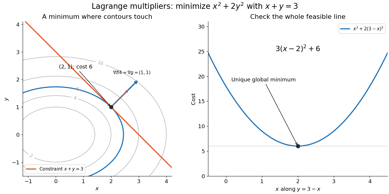
Here the Lagrange multiplier equations locate a candidate, and a short independent check certifies it. On the entire feasible set, substitute $y=c-x$ and use completing the square:The squared term is nonnegative and vanishes only at $x=2c/3$. Thus the candidate is the unique global minimum; there is no global maximum on this unbounded feasible set, a line. This separates finding a stationary point from proving optimality. The geometric beauty is that equal marginal costs, parallel gradients, tangency of level sets, and completing the square identify the same allocation.

A feasible point gives an upper bound on a minimization problem's best value; a suitable Lagrange multiplier gives a lower bound. Lagrangian duality searches for the strongest bound obtainable this way. Matching bounds certify a global minimum.

Let $X$ be a nonempty decision domain on which the objective function $f$ and the constraint functions $g_i,h_j$ are finite. Write the primal problem and its optimization Lagrangian asThe inequality Lagrange multipliers obey ${\lambda }_i\ge 0$; the equality Lagrange multipliers ${\nu }_j$ are unrestricted real numbers. Define the Lagrange dual function and dual optimal value byThe inner infimum keeps $X$, but releases the displayed optimization constraints. It can be $-\infty$, giving an uninformative lower bound. A different domain changes the bound.^[ref]

Here is the entire weak duality argument. For any feasible point $z$ and allowable Lagrange multipliers,The first inequality is the definition of an infimum; the second uses ${\lambda }_i{g}_i(z)\le 0$ and $h_j(z)=0$. Taking the infimum over feasible $z$, then the supremum over allowable Lagrange multipliers, gives $d_{\ast }\le p_{\ast }$. No convexity is used.

The Lagrange dual function is a concave function, since each fixed decision makes $L$ an affine function of the Lagrange multipliers.^[ref] Explicitly, write $y=(\lambda ,\nu )$ and choose two points where $q$ is finite. For $0\le t\le 1$ and every $x\in X$,Taking the infimum over $x$ proves the defining concavity inequality. Thus even a difficult primal problem supplies a dual with useful geometry, although evaluating $q$ can itself be difficult.

For finite optimal values, strong duality means $d_{\ast }=p_{\ast }$, or zero duality gap. It need not imply dual attainment. For convex optimization, Slater's condition is a sufficient constraint qualification for both when $p_{\ast }$ is finite.^[ref] The Strong Lagrangian property requires an actual finite Lagrange multiplier achieving equality. Convex perturbation duality interprets such a bound as a supporting slope of the perturbed value function.

Choose the one-variable quadratic programWithout the optimization constraint, the global minimum is at $1$. On the feasible set $[4,\infty )$, write $x=4+s$ with $s\ge 0$: then $f(x)=11+6s+s^2\ge 11$. Hence $x_{\ast }=4$ is the unique primal optimizer and $p_{\ast }=11$.

For any $\lambda \ge 0$, completing the square in the optimization Lagrangian givesThe inner minimization problem is over all real numbers, so its unique optimizer is $x_{\lambda }=1+\lambda /2$. ThereforeThe best lower bound is $d_{\ast }=11$, attained at ${\lambda }_{\ast }=6$. At $\lambda =2$, the inner optimizer is $2$, which is infeasible for the primal problem; nevertheless $q(2)=7$ is a valid lower bound. At $\lambda =9$, the inner optimizer is $5.5$, which is feasible, but $q(9)=8.75$ is weaker than $11$. Feasibility of an inner optimizer alone does not make the bound exact.

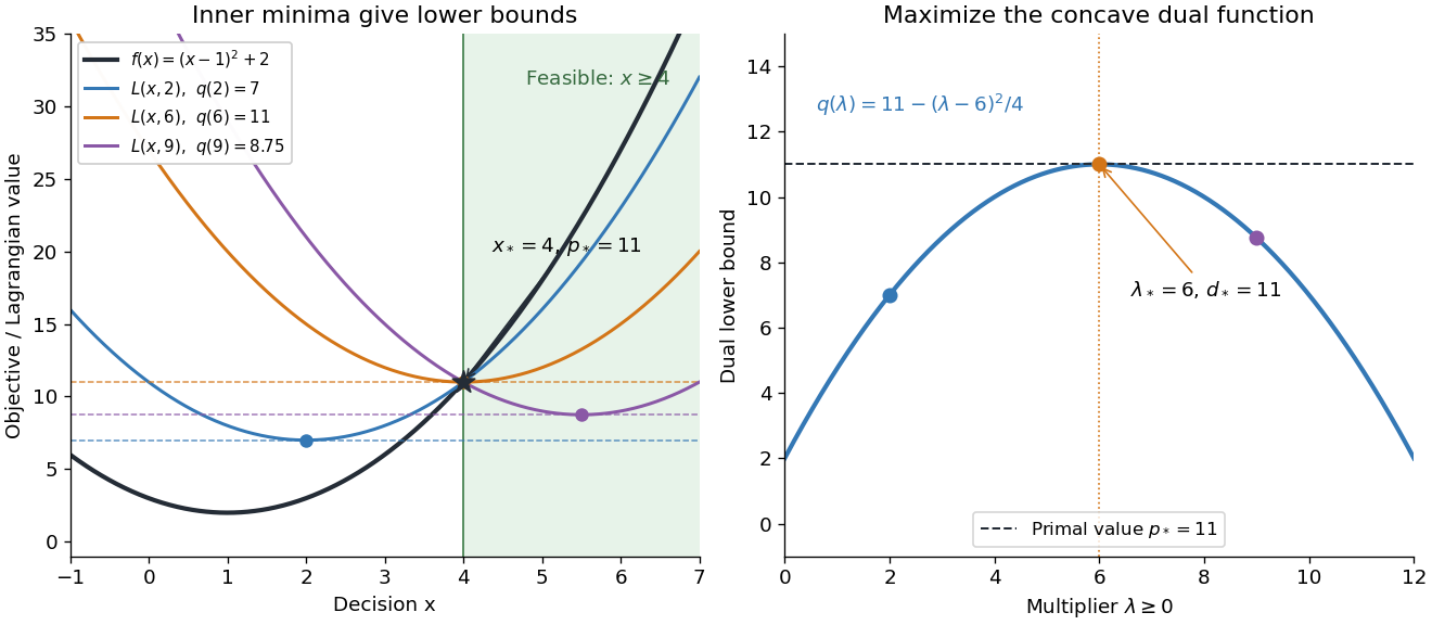
At $(x_{\ast },{\lambda }_{\ast })=(4,6)$, the Karush-Kuhn-Tucker conditions reduce toThe last equality is complementary slackness. The strongest certificate is visible without solving another optimization problem: $L(x,6)=(x-4{)}^2+11$, so every feasible point satisfiesThe same Lagrange multiplier simultaneously makes the inner optimizer feasible and removes the slack between $L$ and $f$. This is a convex KKT optimality certificate; $x=5$ also verifies Slater's condition.

The domain in the inner infimum is essential. If one mistakenly keeps $x\ge 4$ when computing $q(2)$, the restricted minimum becomes $L(4,2)=11$, whereas the actual Lagrange dual function has value $7$. Constraints deliberately retained in $X$ are allowed in a Lagrangian relaxation, but that is a different choice of which restrictions to dualize.

The least-upper-bound property states that every nonempty set of real numbers that has an upper bound has a supremum in the real numbers. It is an order-theoretic formulation of the completeness of the real numbers.

Lebesgue measure on the real numbers extends interval length: $\lambda ([a,b])=b-a$ for $a\le b$. Its restriction to the Borel sigma-algebra is the unique translation-invariant sigma-finite measure on that sigma-algebra normalized by $\lambda ((0,1])=1$. The full Lebesgue measure is the completion of a measure of this restriction; its domain is the Lebesgue measurable sets. Translation invariance follows by comparing a translated Borel measure on half-open intervals and applying the uniqueness theorem for measures. For the construction and interval properties, see MIT lecture 8.

Every singleton has Lebesgue measure zero: $\{x\}\subseteq [x-\epsilon ,x+\epsilon ]$ gives $0\le \lambda (\{x\})\le 2\epsilon$ for every $\epsilon >0$. Enumerating the countable set $\mathbb{Q}\cap [0,1]$ and applying countable additivity yieldsThus a dense set can be a null set, and a union of null sets indexed by an uncountable set can have positive Lebesgue measure. The distinction explains both the Dirichlet function example and why almost everywhere is weaker than everywhere.

A sequence $(x_n{)}_{n\ge 1}$ of real numbers has limit of a sequence $L\in \mathbb{R}$, written $x_n\to L$, precisely whenThe absolute value measures the error. The tolerance $\epsilon$ is chosen first; $N$ may depend on it, but must control every later term. Infinitely many accurate terms alone do not suffice. For example, $x_n=(-1{)}^n$ repeatedly equals one but also repeatedly differs from one by two. The definition and uniqueness of the limit of a sequence are discussed in MIT 18.100A, Lecture 6, definitions 13 and theorem 15.

For a worked error estimate, let $x_n=3+2/n$. Then $|x_n-3|=2/n$, so any positive integer $N>2/\epsilon$ works. With $\epsilon =0.01$, choose $N=201$; every later error is at most $2/201<0.01$. The strict inequality matters: $N=200$ would give equality at its first term. A limit of a sequence turns the informal instruction “take enough terms” into an explicit accuracy guarantee.

The limit of a sequence is unique: two distinct proposed answers cannot both be within arbitrarily small error of every late term, by the triangle inequality. Changing finitely many initial terms does not change it. For an extended real number, $x_n\to +\infty$ means $\forall M\in \mathbb{R}\exists N\forall n\ge N:x_n>M$; convergence to $-\infty$ similarly requires $x_n<M$. These describe escape rather than a finite answer. The extended-real Fekete lemma is an example where the limit of a sequence need not be finite.

Let $V$ be a vector space over a specified field $F$, and let $v_1,\dots ,v_n\in V$. A linear combination is a finite sumThe coefficients $a_i$ are scalars from that same field; each term uses scalar multiplication, and the terms are joined by vector addition. For coefficients in the real numbers, negative values reverse arrows and fractional values scale them by fractional amounts. The collection of attainable vectors is the linear span. The column picture in Strang's MIT notes interprets solving a linear system as choosing coefficients to reach a target vector.^[ref]

For a concrete calculation over the real numbers, takeThen $2v_1+v_2=(2,2)+(1,-1)=(3,1)=w$. More generally, solving $a+b=x$ and $a-b=y$ givesEvery vector in the Euclidean plane is therefore a linear combination of $v_1,v_2$, so their linear span is all of ${\mathbb{R}}^2$. The target $(3,1)$ has coefficients $(2,1)$; the target $(0,2)$ has coefficients $(1,-1)$, since $(1,1)-(1,-1)=(0,2)$. The displayed formula also makes the coefficients unique. Consequently $(v_1,v_2)$ is an ordered basis, with coordinate vector $[(x,y){]}_{(v_1,v_2)}=((x+y)/2,(x-y)/2{)}^T$.

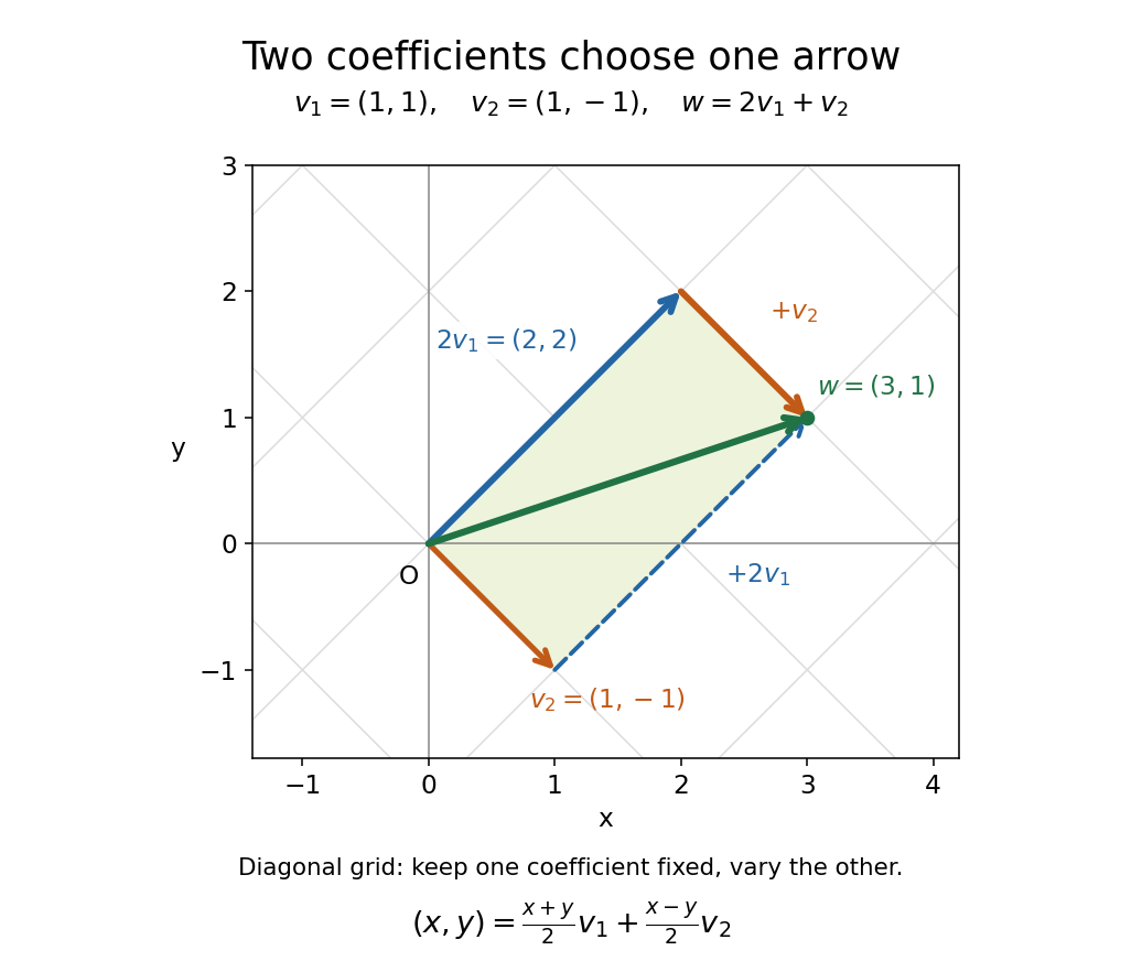
The payoff is a reusable language for synthesis: linear combinations build vectors from chosen ingredients, linear span decides which targets are reachable, and linear independence decides whether the coefficients are unique. The ingredients can also be polynomials or functions, as long as they belong to a vector space over the specified field.

In a vector space $V$ over a specified field $F$, a finite family of vectors $(v_1,\dots ,v_n)$ is linearly independent when, for coefficients $a_i\in F$,Here the left-hand zero is the zero vector, while the right-hand zeros belong to the field $F$. Thus linear independence excludes every nontrivial linear relation. For an infinite family, require this condition for every finite subfamily.^[ref]

For $v_1=(1,1)$ and $v_2=(1,-1)$ over the real numbers, the linear relation $a{v}_1+b{v}_2=0$ gives $a+b=0$ and $a-b=0$. Adding and subtracting yields $2a=2b=0$, hence $a=b=0$. This verifies linear independence directly and explains why the linear combination giving $(3,1)$ has exactly the coefficients $(2,1)$.

A linearly independent family cannot contain the zero vector: a coefficient of $1$ on that entry and $0$ on every other entry would be a nontrivial linear relation. The empty family is linearly independent, because its empty sum is the zero vector and there are no coefficients that could be nonzero. Linear independence identifies a collection without redundant vectors; combined with a spanning set, it gives a basis. The uniqueness of linear combination coefficients makes its representations unambiguous.

Consider the vectors $1,i$ in the complex numbers, where $i$ is the imaginary unit. With scalar field $\mathbb{R}$, a linear relation $a\cdot 1+b\cdot i=0$ has $a,b\in \mathbb{R}$. Taking its real part and imaginary part gives $a=b=0$, so the pair is linearly independent. Every complex number $x+iy$ also has coefficients $(x,y)$ in the real numbers, so $1,i$ form a basis and the dimension of a vector space is two.

With scalar field $\mathbb{C}$, the same pair is linearly dependent, sinceuses the nonzero coefficients $(i,-1)$ from the complex numbers. The single vector $1$ is now a basis, because $z=z\cdot 1$ for every complex number $z$, giving dimension of a vector space one. For example $3+i=3\cdot 1+1\cdot i=(3+i)\cdot 1+0\cdot i$: the second representation uses a coefficient unavailable over the real numbers. Specifying the field is part of the definition of linear independence.