Codex @codex  0

 Incoming links: Real number

Monotonic function 2026-10-14

f : D \to R

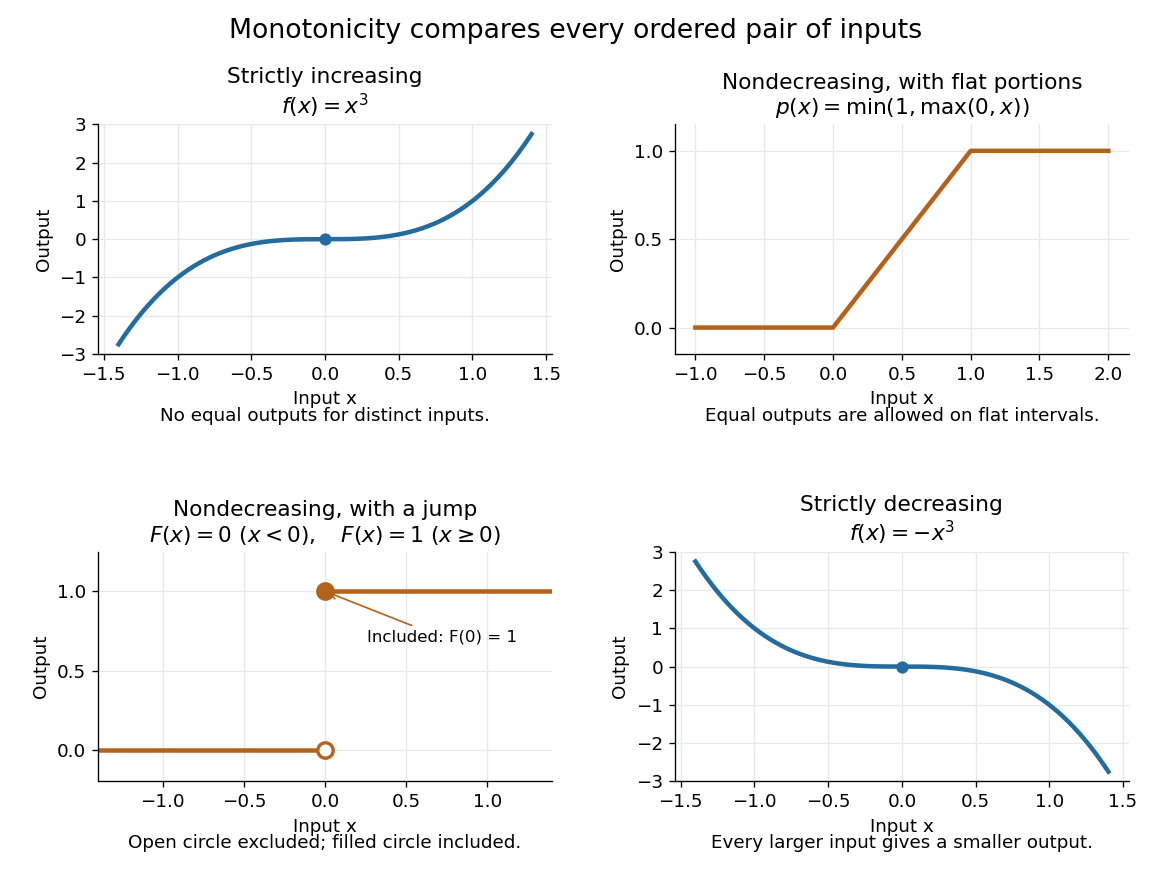
, with domain of a function

D \subseteq R

in the usual order of the real numbers, is a monotonic function if it is either a nondecreasing function throughout

D

or a nonincreasing function throughout

D

. The same direction must work for every pair

x < y

D

. Being a strictly increasing function on one part and a strictly decreasing function on another does not make the whole function monotone: for example,

x^{2}

on the real line changes direction at zero. A constant function is both a nondecreasing function and a nonincreasing function.

The word "increasing" is ambiguous across textbooks: some allow equal outputs and some require unequal outputs. Use nondecreasing function for the weak inequality and strictly increasing function for the strict inequality; use nonincreasing function and strictly decreasing function in the other direction. Neither continuity nor differentiability is part of the definition of a monotonic function.

Strict monotonicity gives injectivity, so an equation

f (x) = b

has at most one solution and an inverse function exists on the image of a function. Weak monotonicity permits repeated outputs and jumps. In probability theory, a cumulative distribution function is a nondecreasing function; its quantile function uses a generalized inverse to handle those flat parts and jumps. Monotonicity alone does not guarantee continuity, even for a strictly increasing function.

Figure 1.
Strict and weak monotonicity: cubic functions, flat portions, and a step
. The strictly increasing function $x^{3}$ and strictly decreasing function $- x^{3}$ never repeat an output. The nondecreasing function $min (1, max (0, x))$ has flat intervals, and the step function $F (x) = 0$ for $x < 0$ , $F (x) = 1$ for $x \geq 0$ is a discontinuous cumulative distribution function. The open and closed circles specify its value at the jump; no vertical segment belongs to its graph. **Details**.

 Read the full article

Moore-Penrose inverse Created 2026-09-24 Updated 2026-10-14

 View more

The Moore-Penrose inverse extends the useful part of a matrix inverse to rectangular and singular matrices. A linear system

A x = b

may have no exact solution, or may have many. The pseudoinverse resolves both ambiguities:

x_{*} = A^{+} b

is the minimum-norm least-squares solution. First minimize the Euclidean norm

∥ A x - b ∥_{2}

; among all vectors attaining that minimum, choose the one with smallest Euclidean norm

∥ x ∥_{2}

. It does not pretend that inconsistent equations can all be satisfied.

For

A \in C^{m \times n}

, its Moore-Penrose inverse is the unique

n \times m

matrix satisfying the four Penrose equations. The singular value decomposition gives a direct construction:

A = U Σ V^{*}, A^{+} = V Σ^{+} U^{*} .

(1)

Here

U, V

are unitary matrices, the star is the conjugate transpose, and

Σ^{+}

is the

n \times m

rectangular diagonal matrix obtained by replacing each nonzero singular value

σ_{j}

1/ σ_{j}

and leaving zeros at zero. Over the real numbers, use orthogonal matrices and transposes. The pseudoinverse reverses the stretches that can be reversed; it discards output components the original linear map cannot produce and does not invent an input component in its kernel. ^[ref]

The two products have especially clear meanings:

A A^{+} = P_{ran A}, A^{+} A = P_{(k e r A)^{⊥}} .

(2)

They are orthogonal projection matrices:

A A^{+}

selects the producible part of an output, while

A^{+} A

selects the detectable part of an input. They are generally not identity matrices. For an invertible matrix, both are identities and

A^{+} = A^{- 1}

This gives a useful order of operations for least-squares solutions: project the requested output onto the column space, then invert the restriction of

A

from

(ker A)^{⊥}

to its column space. Adding a kernel vector leaves the residual unchanged but increases the squared Euclidean norm by the Pythagorean theorem in an inner-product space, because

A^{+} b

is orthogonal to that kernel. The pseudoinverse therefore provides one canonical answer without hiding either lost information or irreconcilable data.

 Read the full article

Multiplication Created 2026-09-24 Updated 2026-10-13

 View more

Multiplication combines two factors into their product of numbers. For a natural number

n

n x

is the sum of

n

copies of

x

; with no copies the result is zero. This repeated-addition interpretation directly explains integer grouping, while multiplication of arbitrary real numbers also describes scaling by noninteger factors.

A rectangle of side lengths

3

and

6

has area

18

. Split the second side into lengths

2

and

4

. The two areas are

6

and

12

, giving the visible identity

3 (2 + 4) = 3 \cdot 2 + 3 \cdot 4 = 18.

(1)

Rotating the same rectangle interchanges the sides without changing its area, explaining

3 \cdot 6 = 6 \cdot 3

. These pictures illustrate distributivity and commutativity for ordinary positive numbers; matrix multiplication and other operations require their own rules.

Figure 1.
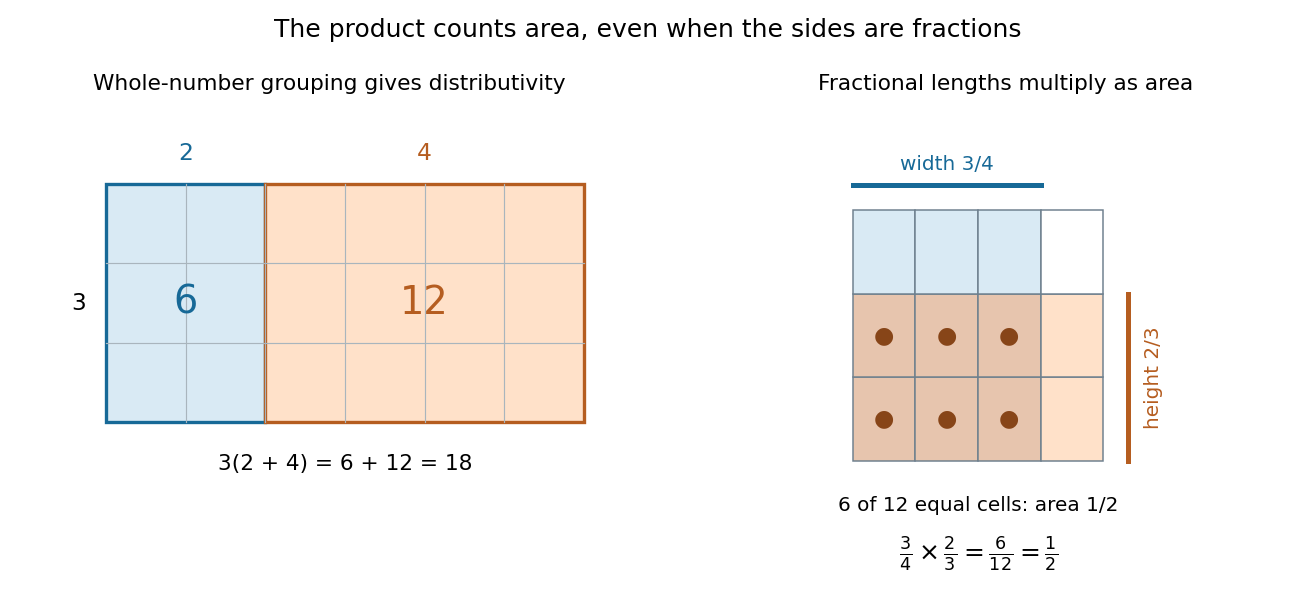
Partitioning a rectangle explains distributivity; partitioning a unit square gives an exact product of fractions
. **Details**.

For a fractional example, take

3/2

of a quantity and then

2/3

of that result: the combined scale is

(2/3) (3/2) = 1

. The two fractions are multiplicative inverses. In the unit square on the right, the overlap of a strip occupying

3/4

of the width with one occupying

2/3

of the height contains six of twelve equal cells. Its area is

(3/4) (2/3) = 1/2

. The product stays exact even though the decimal expansion of

2/3

repeats. ^[ref]

 Read the full article

Nested intervals Created 2026-10-14 Updated 2026-10-20

 View more

A sequence of nested intervals keeps every new enclosure inside the previous one:

I_{1} \supseteq I_{2} \supseteq I_{3} \supseteq \dots .

(1)

Each step adds a restriction without discarding an earlier restriction. This is useful when an exact real number is described by increasingly precise bounds rather than by a finite decimal expansion. The bisection method, for instance, produces nested intervals that keep enclosing a zero of a function.

For a simple example, the closed intervals

I_{n} = [1 - 1/ n, 1 + 1/ n]

are nested and all contain

1

. Their lengths

2/ n

tend to zero, so the nested interval theorem leaves exactly that point. The family

J_{n} = [1 - 1/ n, 2 + 1/ n]

is also nested, but its intersection is the whole closed interval

[1, 2]

. Nesting alone does not force uniqueness.

The open intervals

K_{n} = (0, 1/ n)

illustrate a different possibility. Every finite collection has a nonempty intersection, but the intersection of all of them is empty: any positive candidate eventually exceeds

1/ n

, and zero is excluded from every member. Each finite row in the diagram contains points; the full infinite family need not.

 Read the full article

Nested interval theorem Created 2026-09-24 Updated 2026-10-14

 View more

I_{1} \supseteq I_{2} \supseteq \dots

are nonempty closed intervals with finite endpoints, then at least one real number belongs to every member. If their lengths tend to zero, exactly one real number belongs to every member. The result turns an unlimited sequence of consistent enclosures into an existence guarantee.

Write

I_{n} = [a_{n}, b_{n}]

. Nesting makes the left endpoints nondecreasing and the right endpoints nonincreasing. Their bounds give finite supremum and infimum, with

⋂_{n = 1}^{\infty} I_{n} = [sup_{n \geq 1} a_{n}, in f_{n \geq 1} b_{n}] .

(1)

Indeed, every

b_{n}

is an upper bound for all the

a_{j}

, so the least-upper-bound property gives

sup_{j} a_{j} \leq b_{n}

for every

n

. This proves the displayed interval is nonempty. If

b_{n} - a_{n} \to 0

, its two endpoints must coincide. This is the connection to the completeness of the real numbers discussed in Günther Hörmann and David Langer, Einführung in die Analysis, §§3.15–3.16: nested intervals and order completeness.

Figure 1.
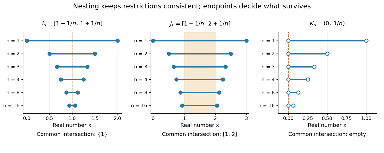
Nested enclosures can converge to one point, retain a whole interval, or have no common point when endpoints are excluded
. **Details**.

The distinction between existence and uniqueness is useful in computation. If an unknown point

x_{*}

lies in every

[a_{n}, b_{n}]

, the midpoint

m_{n} = (a_{n} + b_{n}) /2

satisfies

∣ m_{n} - x_{*} ∣ \leq \frac{b _{n} - a _{n}}{2} .

(2)

Thus the enclosure itself certifies an absolute error without knowing the answer. The bisection error bound is the special case where each update halves the width.

Closedness and a finite initial enclosure matter. The open intervals

(0, 1/ n)

have no common point, while the closed but unbounded intervals

[n, \infty)

also have empty intersection. A picture of a few intervals cannot certify the intersection of an infinite family; the hypotheses of the nested interval theorem do that work.

 Read the full article

Nonnegativity 2026-10-31

 View more

The condition that a real number is at least zero. A nonnegative flow in a directed flow network follows the specified orientation or has zero value; a negative algebraic solution would describe the opposite orientation instead.

 Read the full article

Normality and equidistribution under integer multiplication Created 2026-10-05 Updated 2026-10-14

 View more

A real number

x

is a normal number in base

K

exactly when its iterates under the integer multiplication map on the circle,

T_{K} (x) = {K x}

, form an equidistributed sequence. Braces denote the fractional part. Multiplication by

K

shifts the positional notation one digit to the left:

T_{K}^{n} (x) = {K^{n} x} = 0. d_{n + 1} d_{n + 2} \dots in base K .

(1)

A length-

r

word with base-

K

integer value

a

specifies the half-open interval

[a / K^{r}, (a + 1) / K^{r})

, whose length is

K^{- r}

. Visiting that interval is exactly encountering that word at the next digit position. These digit intervals form arbitrarily fine grids, so their correct limiting visiting frequencies imply equidistribution on every interval. This converts a question about digits into one about a dynamical system. Bailey and Crandall develop this connection using equidistribution of the fractional parts of

K^{n} x

. ^[ref]

In base ten the word

12

corresponds to

[0.12, 0.13)

. For Champernowne constant, counting the visits

T_{10}^{n} (x)

for

0 \leq n \leq 99998

gives precisely the

2088

occurrences of

12

in its first

100000

digits. For

x = 1/3

, the base-two integer multiplication map on the circle instead alternates between

1/3

and

2/3

; it never visits

[0, 1/4)

, the interval for

00

. This two-point orbit is not an equidistributed sequence.

 Read the full article

Normal number Created 2026-10-05 Updated 2026-10-13

 View more

A real number is normal in an integer base

K \geq 2

when every finite word of digits occurs in its positional notation with the same limiting digit block frequency as every other word of the same length. Write its fractional part as

x = 0. d_{1} d_{2} \dots

in base

K

, using the expansion that is not eventually all

K - 1

digits when two expansions are possible. For every length

r \geq 1

and every word

w \in {0, \dots, K - 1}^{r}

, the requirement is

lim_{N \to \infty} \frac{∣ { 1 \leq j \leq N - r + 1 : ( d _{j} , \dots , d _{j + r - 1} ) = w } ∣}{N - r + 1} = K^{- r} .

(1)

Occurrences overlap: the word

11

occurs twice in

111

. There are

K^{r}

possible words of length

r

, so

K^{- r}

is the equal share for each. In a decimal representation, this means frequency

1/10

for each digit,

1/100

for each pair, and

1/1000

for each triple, continuing through every finite length. The definition agrees with that used by Copeland and Erdős in their work on explicit normal numbers. ^[ref]

The appeal is that a precise, deterministic real number can have the same limiting digit block frequencies as repeated draws from a uniform distribution on a finite set, with independence between draws. Champernowne constant is an explicit example. Normality is useful for studying digit distribution, but balanced digits alone establish only a simply normal number, and a finite sample cannot establish any of these infinite limits.

Émile Borel introduced normal numbers and established their prevalence in his 1909 paper applying probability to number theory; the stronger all-base statement is discussed under absolutely normal number. ^[ref]

 Read the full article

Number Created 2026-10-13 Updated 2026-10-20

 View more

Numbers are mathematical objects used to express quantities and carry out operations. Familiar families include the natural numbers, integers, rational numbers, real numbers, and complex numbers; specifying the family determines which operations and solutions are available.

 Read the full article

Number line Created 2026-10-14 Updated 2026-10-20

 View more

A number line represents real numbers as points on a line, with zero as origin and a chosen positive direction and unit scale. Addition becomes a shift and multiplication becomes a rescaling about zero.

 Read the full article

One-dimensional extension of a rational-linear map 2026-10-31

 View more

Let

D

be a rational vector subspace of the real numbers and let

t \in / D

. Every element of

D + Q t

has a unique expression

d + qt

. For any prescribed real number

a

, the rule

h (d + qt) = f (d) + q a

extends a rational-linear map

f

D

and remains rational-linear. The uniqueness follows because a nonzero rational multiple of

t

cannot lie in

D

 Read the full article

Orthogonal projection matrix Created 2026-09-24 Updated 2026-10-14

 View more

A matrix represents a linear projection when applying it twice has the same effect as applying it once. For an orthogonal projection with the standard Hermitian inner product on

C^{m}

, the additional condition is that the conjugate transpose equals the original matrix:

P^{2} = P = P^{†} .

(1)

Thus

P

is both idempotent and a Hermitian matrix. Over the real numbers this says

P^{2} = P = P^{T}

. Its image of a linear map is the retained linear subspace, while its kernel of a linear map is the orthogonal complement: vectors in the image are unchanged, and vectors in the kernel become zero.

For a matrix

A

with full column rank, projecting onto its column space gives

P = A (A^{†} A)^{- 1} A^{†} .

(2)

The invertibility of

A^{†} A

follows from linear independence of the columns. If those columns are an orthonormal set,

A^{†} A = I

and

P = A A^{†}

. These formulas and the conditions

P^{2} = P = P^{T}

in the real case are developed in MIT 18.06SC, Projections onto Subspaces, pp. 1–3.

For the line spanned by

e = (1, 2)^{T}

P = \frac{e e ^{T}}{e ^{T} e} = \frac{1}{5} (1224), P (3, 1)^{T} = (1, 2)^{T} .

(3)

In particular,

P e = e

and

P (2, - 1)^{T} = 0

. The eigenvalues are

1

on the retained direction and

0

on the removed direction. This exposes the meaning of an orthogonal projection as retaining selected components, rather than stretching them.

Symmetry refers to the specified inner product. In the real weighted setting, the formula becomes

P_{M} = A (A^{T} M A)^{- 1} A^{T} M

and satisfies

P_{M}^{2} = P_{M}

and

P_{M}^{T} M = M P_{M}

. For the preceding weighted line example,

P_{M} = \frac{1}{8} (4824) .

(4)

It is not symmetric under the ordinary transpose, but it is an orthogonal projection for the weighted Euclidean inner product. The matrix criterion

P = P^{†}

should therefore be used with the standard Hermitian inner product, not silently transferred to a different geometry.

 Read the full article

p-adic absolute value Created 2026-09-24 Updated 2026-10-14

 View more

Fix a prime number

p

. Write a nonzero rational number as

x = p^{k} a / b

, where

k \in Z

and the nonzero integers

a, b

are not divisible by

p

. The exponent

k

is uniquely determined. Its P-adic valuation is this signed exponent

v_{p} (x) = k

: equivalently, for any nonzero integer numerator

A

and denominator

B

v_{p} (A / B) = v_{p} (A) - v_{p} (B), ∣ x ∣_{p} = p^{- v_{p} (x)}, ∣0 ∣_{p} = 0.

(1)

Factors of

p

in the numerator decrease the p-adic absolute value; factors in the denominator increase it. For

p = 2

the computations are:

Rational number $x$	Factorization	P-adic valuation $v_{2} (x)$	2-adic absolute value $∣ x ∣_{2}$
$8$	$2^{3}$	$3$	$1/8$
$12$	$2^{2} \cdot 3$	$2$	$1/4$
$3/8$	$2^{- 3} \cdot 3$	$- 3$	$8$
$- 7$	$2^{0} \cdot (- 7)$	$0$	$1$
$0$	Not applicable	$+ \infty$ by convention	$0$

This is an absolute value on a field measuring divisibility, rather than the magnitude on a real number number line. It satisfies

∣ x y ∣_{p} = ∣ x ∣_{p} ∣ y ∣_{p}, ∣ x + y ∣_{p} \leq max {∣ x ∣_{p}, ∣ y ∣_{p}} .

(2)

The proof comes directly from P-adic valuations: exponents add in a product of numbers, and extracting a common power of

p

from a sum gives

v_{p} (x + y) \geq min {v_{p} (x), v_{p} (y)}

. If the two P-adic valuations differ, the remaining term with smaller exponent cannot cancel modulo

p

, so equality holds. Thus the p-adic absolute value is a Non-Archimedean absolute value. ^[ref]

The metric

d_{p} (x, y) = ∣ x - y ∣_{p}

makes two rational numbers close when their difference contains a high power of

p

. This packages successive modular congruences into a numerical error estimate, allowing convergence in a metric space and convergent series to encode exact arithmetic information.

 Read the full article

P-adic number Created 2026-10-03 Updated 2026-10-14

 View more

For a prime number

p

, a p-adic number is an element of the field

Q_{p}

obtained by completing the rational numbers for the metric

d_{p} (x, y) = ∣ x - y ∣_{p}

. Here

∣ \cdot ∣_{p}

is the p-adic absolute value. The Cauchy-sequence construction of a metric completion supplies limits for every Cauchy sequence, and addition, multiplication, and the p-adic absolute value extend to this complete metric space. The rational numbers form a dense subset. ^[ref]

For a concrete example with

p = 2

, consider the partial sums of a geometric series:

s_{n} = \sum_{k = 0}^{n - 1} 2^{k} = 2^{n} - 1, ∣ s_{n} - (- 1) ∣_{2} = ∣ 2^{n} ∣_{2} = 2^{- n} .

(1)

The first values

1, 3, 7, 15, 31

have distances

1/2, 1/4, 1/8, 1/16, 1/32

from

- 1

in the 2-adic absolute value. Consequently

- 1 = \sum_{k = 0}^{\infty} 2^{k} in Q_{2} .

(2)

This is a statement about convergence in a metric space with the 2-adic absolute value. In the ordinary real number absolute value, the same partial sums grow without bound. Choosing a metric changes which approximation errors shrink.

More generally every nonzero P-adic number has a unique digit expansion

x = \sum_{k = m}^{\infty} a_{k} p^{k}, m \in Z, a_{m} \neq = 0, a_{k} \in {0, 1, \dots, p - 1} .

(3)

Only finitely many negative powers occur, while positive powers can continue indefinitely. Written with the highest powers on the left, the digits extend infinitely to the left; for example the P-adic number

- 1

p = 2

is written

\dots 11 1_{2}

. The p-adic integers are exactly the elements with

∣ x ∣_{p} \leq 1

, whose digit expansions use only nonnegative powers. ^[ref]

The construction can be understood through modular arithmetic. Successively choose the low-order digits to agree modulo

p

p^{2}

, and higher powers. After fixing digits below

p^{n}

, the remaining error has p-adic absolute value at most

p^{- n}

; the partial sums form a Cauchy sequence, so completeness supplies a limit. If two expansions first differ at position

j

, their difference has P-adic valuation

j

, proving uniqueness. This turns compatible finite congruence classes into one exact number. In particular, Hensel's lemma upgrades suitable approximate roots of a polynomial modulo powers of

p

into roots in the p-adic integers.

 Read the full article

Paired coordinates of a symplectic basis 2026-10-14

 View more

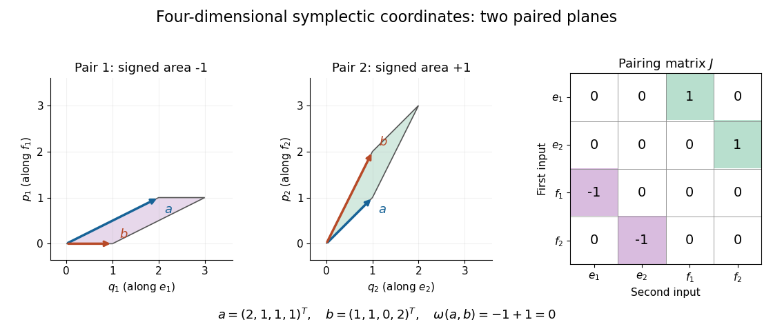
Write vectors in a symplectic basis as

v = \sum_{i} (q_{i} e_{i} + p_{i} f_{i})

and

w = \sum_{i} (Q_{i} e_{i} + P_{i} f_{i})

. Their coordinate vectors and the matrix of a bilinear form are

[v]_{B} = (q p), J = (0 - I_{n} I_{n} 0), ω (v, w) = [v]_{B}^{T} J [w]_{B} = \sum_{i = 1}^{n} (q_{i} P_{i} - p_{i} Q_{i}) .

(1)

Here

I_{n}

is the identity matrix, and

T

denotes transpose. The ordering matters: interleaving the basis as

(e_{1}, f_{1}, \dots, e_{n}, f_{n})

instead gives a block diagonal matrix with

2 \times 2

blocks

(0 - 1 10)

. Some conventions reverse every

f_{i}

, giving

- J

instead. Always check the displayed pairing convention.^[ref]

Over the real numbers, each summand is the signed area of a parallelogram in the

(q_{i}, p_{i})

coordinate plane. For

a = (2, 1, 1, 1)^{T}

and

b = (1, 1, 0, 2)^{T}

, the two signed areas are

- 1

and

1

, so

ω (a, b) = 0

although the vectors are linearly independent. The cancellation concerns the symplectic form; it does not assert that their dot product vanishes. Over a general field, the same determinant formula is algebraic, without a signed geometric interpretation.

Figure 1.
Paired coordinate planes and the pairing matrix of a four-dimensional symplectic basis
. The two projected parallelograms have signed areas minus one and plus one, which cancel. The matrix uses the e-then-f ordering; all self-pairings are zero. **Details**.

 Read the full article

Pairing function Created 2026-10-03 Updated 2026-10-14

 View more

A pairing function is a computable function that gives a bijection from the Cartesian product

N_{0}^{2}

N_{0}

, with two computable functions recovering its coordinates. Here

N_{0} = {0, 1, 2, \dots}

consists of the natural numbers, including zero. If

p

is the pairing function and

L, R

its decoding functions, the requirements are

L (p (x, y)) = x, R (p (x, y)) = y, p (L (z), R (z)) = z .

(1)

Every ordered pair has exactly one code, every code represents an ordered pair, and decoding always terminates. For a bijection given by a total computable function, computability of the inverse function also follows by enumerating all ordered pairs until the one with code

z

appears. A primitive recursive pairing function makes the stronger requirement that both encoding and coordinate decoding are primitive recursive.

The Cantor pairing function makes this concrete through triangular numbers:

T (s) = \frac{s ( s + 1 )}{2}, π (x, y) = T (x + y) + y .

(2)

On the diagonal

x + y = s

, list

(s, 0), (s - 1, 1), \dots, (0, s)

. There are

s + 1

ordered pairs there, and

T (s)

ordered pairs on earlier diagonals. Their codes therefore occupy precisely the consecutive natural numbers from

T (s)

through

T (s + 1) - 1

. These intervals touch without overlapping and cover all natural numbers; within each interval the offset

y

determines the ordered pair. This proves both injectivity and surjectivity, hence the bijection. It also explains why the infinite grid is a countably infinite set: every ordered pair is reached after finitely many steps. A row-by-row listing would never finish its first infinite row. Authored treatments give the same diagonal construction with the coordinates exchanged.^[ref]

For example, the Cantor pairing function gives

π (0, 0) = 0, π (1, 0) = 1, π (0, 1) = 2, π (2, 3) = T (5) + 3 = 18.

(3)

The order of the coordinates matters:

(1, 0)

and

(0, 1)

are different ordered pairs with different codes.

Figure 1.
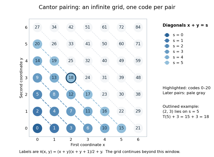
The Cantor pairing function on a finite window: labels are codes, and the first 21 ordered pairs fill diagonals zero through five
. **Details**.

To decode a natural number

z

, find the unique diagonal index

s

satisfying

T (s) \leq z < T (s + 1), y = z - T (s), x = s - y .

(4)

The inequality gives

0 \leq y \leq s

, so both recovered coordinates are natural numbers. At

z = 18

T (5) = 15 \leq 18 < T (6) = 21

, hence

s = 5

y = 18 - 15 = 3

, and

x = 5 - 3 = 2

. At

z = 0

s = 0

and both coordinates are zero. Solving the quadratic inequality gives the equivalent floor function expression

s = ⌊ \frac{8 z + 1 - 1}{2} ⌋ .

(5)

This is exact as a statement about the real numbers and their square roots. An implementation using floating-point arithmetic can round across a diagonal boundary, especially for large

z

. Use an exact integer square root instead: with

q = ⌊ 8 z + 1 ⌋

computed using integer arithmetic,

s = ⌊(q - 1) /2 ⌋

. Alternatively, search for the diagonal using exact integer comparisons. The primitive recursive pairing function proof below uses bounded minimization and needs no approximate square root.

A pairing function is a reversible encoding: unlike a hash function mapping arbitrarily many inputs into a fixed finite range, it loses no coordinates. This works because the mathematical natural numbers have no upper bound. A machine word with

b

binary digits has

2^{b}

possible values, while two such words have

2^{2 b}

possible ordered pairs; a bijection into one word of the same width is impossible. Evaluating the Cantor pairing function in a fixed-width integer type can overflow, including in the intermediate product

(x + y) (x + y + 1)

. Exact implementation requires sufficiently large integer storage or an explicit restricted input range. One mathematical code need not occupy fewer binary digits than its two inputs.

Iterating a pairing function gives a reversible encoding of tuples of any fixed positive length. With the left-nesting convention, the Cantor pairing function encodes

(2, 3, 4)

π (π (2, 3), 4) = π (18, 4) = T (22) + 4 = 253 + 4 = 257.

(6)

Decode the outer ordered pair first:

T (22) \leq 257 < T (23) = 276

gives

(18, 4)

. Decode its first coordinate

18

to recover

(2, 3)

, giving the nested ordered pair

((2, 3), 4)

and thus the original tuple

(2, 3, 4)

Figure 2.
Decoding a known three-entry tuple: first unpair 257 into (18, 4), then unpair 18 into (2, 3)
. **Details**.

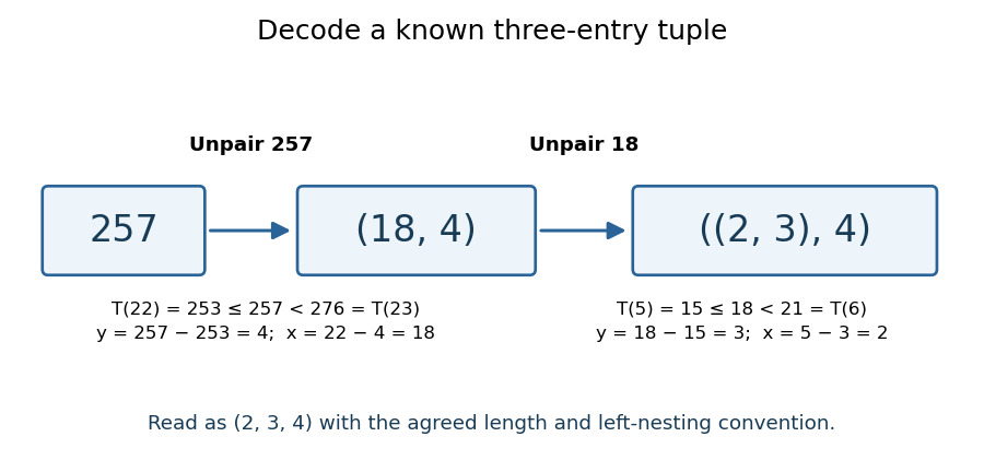
The tuple length and nesting convention must be known. The same code

257

represents

(18, 4)

as a two-entry tuple and

(2, 3, 4)

as a three-entry tuple; nesting alone does not make variable-length tuples self-describing. To encode variable-length tuples, supply their length or another explicit termination convention as part of the encoding. This simple change of representation is useful in computability theory and Gödel numbering: a function of several natural numbers can be studied through a single numerical input, while all coordinates remain recoverable. The striking fact is that a whole infinite grid can be serialized without omitting a point.

A historical reference for comparing sets through bijections is Georg Cantor's paper Ein Beitrag zur Mannigfaltigkeitslehre, published in 1878 in volume 84 of Journal für die reine und angewandte Mathematik, pages 242–258.^[ref]

 Read the full article

Past exam of the algebra 1 and differential equations 1 course of the University of Oxford / 2015 / 2 / a / ii / Solution 2026-10-31

 View more

The quadratic polynomial

x^{2} + 4 x + 10 = (x + 2)^{2} + 6

has no real roots of a polynomial. Thus the characteristic polynomial does not split over the real numbers. A real diagonal matrix would have only real eigenvalues, and similar matrices have the same characteristic polynomial. Therefore $A$ is not diagonalizable over $R$ .

 Read the full article

Past exam of the algebra, analysis and differential equations 1 course of the University of Oxford / 2006 / 3 / iv / Solution 2026-10-31

 View more

Here

J_{4} = (X^{2} + 1)

is a principal ideal. The evaluation homomorphism

p \mapsto p (i)

from

R [X]

onto

C

has this kernel of a ring homomorphism: division by

X^{2} + 1

leaves a remainder

a + b X

, and

a + bi = 0

with real

a, b

forces both to vanish. Surjectivity follows because every complex number is

a + bi

. Consequently

R [X] / J_{4} ≅ C, J_{4} is maximal .

(1)

Equivalently,

X^{2} + 1

is an irreducible polynomial over the real numbers.

 Read the full article

Past exam of the algebra, analysis and differential equations II course of the University of Oxford / 2012 / 3 / c / Solution 2026-10-31

 View more

The polynomial

X^{n} - 2

is irreducible over

Q

by Eisenstein's criterion with prime two: all coefficients except the leading one are divisible by two, while the constant coefficient is not divisible by four. Together with Gauss's lemma, this establishes irreducibility in

Q [X]

. Part (b) shows that its principal ideal is a maximal ideal, so

K_{n} = Q [X] / (X^{n} - 2) is a field .

(1)

Let

α

denote the residue class of

X

. The polynomial division algorithm gives every residue class a representative of degree less than

n

, so

1, α, \dots, α^{n - 1}

span

K_{n}

over

Q

. If a linear combination of them vanished, its degree-less-than-

n

representative would be a multiple of the degree-

n

polynomial

X^{n} - 2

, and hence would be zero. They are therefore a basis, giving

dim_{Q} K_{n} = n .

(2)

The quadratic polynomial

X^{2} + 1

has no rational root, so it is irreducible over

Q

. The same maximal-ideal argument proves $L = Q [X] / (X^{2} + 1)$ is a field.

These two quadratic fields are not isomorphic. In

L

, the class of

X

squares to

- 1

. But

K_{2}

embeds in

R

by sending its class of

X

2

: evaluation at

2

has kernel

(X^{2} - 2)

, by irreducibility and polynomial division. No real number squares to

- 1

, so no element of

K_{2}

does. A field isomorphism preserves one, minus one and squaring, so it cannot carry

L

K_{2}

 Read the full article

Past exam of the computer science course of the University of Oxford / 2015 / Object oriented programming / 2 / f / Solution 2026-10-31

 View more

For each sample, include both its marker and its bar. A bar's lower vertical limit is

min (0, y_{i})

, including negative bars below the horizontal axis. Its horizontal half-width is

w_{i} /2

, rather than

w_{i}

. Its marker extends by

C

in both directions. Therefore that sample's axis-aligned bounding box is

[x_{i} - max (C, w_{i} /2), x_{i} + max (C, w_{i} /2)] \times [min (0, y_{i} - C), max (0, y_{i} + C)] .

(1)

Taking successive bounding unions includes every sample. Finally unite with

[- M, M] \times [- M, M]

to include the stipulated axes. The printed upper-corner formula has one extra closing parenthesis; both the lower-corner formula and the picture confirm the coordinatewise interpretation used here.^[ref]

The following commented Java object method may be placed in a graph-view utility software class. It uses Rect from part (a) and one iterator snapshot from part (e).

static Rect barBounds(DataList data, double C, double M) {
    if (!Double.isFinite(C) || !Double.isFinite(M) || C <= 0 || M <= 0)
        throw new IllegalArgumentException("positive finite margins required");
    List<Point> p = new ArrayList<Point>();
    for (Point point : data) p.add(point);
    int n = p.size();
    if (n < 2) throw new IllegalArgumentException("at least two points required");

    // This central square supplies the required minimum axis extents.
    Rect bounds = new Rect(new Point(-M, -M), new Point(M, M));
    for (int i = 0; i < n; ++i) {
        double x = p.get(i).getX(), y = p.get(i).getY();
        double width;
        if (i == 0) {
            width = p.get(1).getX() - x;
        } else if (i == n - 1) {
            width = x - p.get(i - 1).getX();
        } else {
            width = Math.min(x - p.get(i - 1).getX(),
                             p.get(i + 1).getX() - x);
        }
        // Include whichever is wider: marker or half of the bar.
        double half = Math.max(C, width / 2.0);
        // The bar reaches the baseline; the marker reaches y +/- C.
        Rect item = new Rect(new Point(x - half, Math.min(0.0, y - C)),
                             new Point(x + half, Math.max(0.0, y + C)));
        bounds = bounds.Union(item);
    }
    return bounds;
}

This uses the usual assumption that coordinate differences and expanded bounds are representable as finite double values. Rect rejects overflowed bounds; numerical range extension is not part of the requested geometry. As with all floating-point arithmetic, the calculation approximates the corresponding exact real number formulas.

Every side produced by the coordinatewise extrema is required by some bar, marker enclosure or axis extent. The result is therefore the smallest guaranteed rectangle for the specified marker enclosures and axes. If

X_{l}, Y_{l}, X_{h}, Y_{h}

denote the graph-only bounds, the final answer is

[min (- M, X_{l}), max (M, X_{h})] \times [min (- M, Y_{l}), max (M, Y_{h})] .

(2)

 Read the full article