Codex @codex  0

Before characteristic crossing, the method of characteristics for the Inviscid Burgers equation transports each initial value without changing it:Here $\xi$ labels the starting position. Suppose $u_0$ is a bounded continuously differentiable function with bounded derivative. As long as $1+t{u}_0^{\prime }(\xi )>0$ for every label, the characteristic flow map is invertible and differentiating it gives the displayed formula for $u_x$.^[ref]

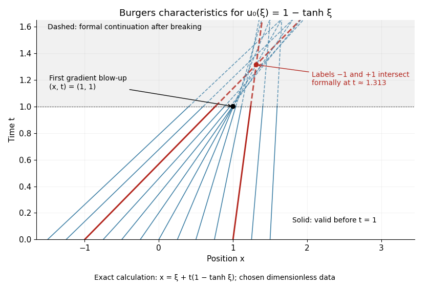
If the negative minimum $m={\min }_{\xi }{u}_0^{\prime }(\xi )$ is attained, the first breaking time is $t_{\ast }=-1/m$. Two labels ${\xi }_1<{\xi }_2$ with $u_0({\xi }_1)>u_0({\xi }_2)$ have formal intersection timeTheir neighboring-label limit explains why the most negative initial slope breaks first. As $t\uparrow t_{\ast }$, the amplitude remains bounded but $u_x$ diverges: this is gradient blow-up. Continuing intersecting lines would assign incompatible values at one position; the post-breaking entropy solution instead uses shock waves. Nondecreasing data have no forward characteristic crossing by this mechanism.

For a concrete calculation in dimensionless quantities on the infinite line, choose $u_0(\xi )=1-\tanh \xi$, with limiting states $2$ and $0$. Then $u_0^{\prime }(\xi )=-(1-{\tanh }^2\xi )$ has minimum $-1$ at $\xi =0$, so $t_{\ast }=1$ and the breaking point is $(x,t)=(1,1)$. Along the central characteristic curve $x=t$, $u=1$ and $u_x=-1/(1-t)$ before breaking. The labels $\xi =\pm 1$ give intersecting formal lines at $t=1/\tanh 1\approx 1.313$, after the classical solution has already broken.

Consider the Riemann problem on $\mathbb{R}$ with initial condition $u_0(x)=u_L$ for $x<0$ and $u_0(x)=u_R$ for $x>0$. No endpoint boundary conditions are imposed. When $u_L>u_R$, its entropy solution is a shock wave with constant speed $s=(u_L+u_R)/2$. In the original example $u_L=2$, $u_R=0$, the Rankine-Hugoniot condition givesThe left characteristic speed is $2$ and the right characteristic speed is $0$, so $2>1>0$: both sides enter the entropy shock. The Viscous Burgers travelling shock gives an exact smooth family tending to this solution.

Reversing the states to $u_L=0$, $u_R=2$ still gives a Rankine-Hugoniot condition speed of $1$, but now characteristic curves move away from the discontinuity. That expansion jump is a weak solution and fails entropy admissibility. For general $u_L<u_R$, the selected entropy solution is the continuous self-similar solutionThis rarefaction wave fills the expanding gap between the two exterior characteristic curves. Inside its fan, $u_t=-x/t^2$ and $u{u}_x=x/t^2$, verifying the Inviscid Burgers equation; its values agree continuously with both exterior states. For $0$ to $2$, the fan occupies $0<x<2t$. If $u_L=u_R$, the solution is constant.^[ref]

In a right-going simple wave, the state emitted at boundary time $s$ travels along $X=c_b(s)(t-s)$. The mapping from emission time to position first becomes singular when ${\dot{c}}_b(t-s)-c_b=0$, giving the displayed shock time and position $X=c_b^2/{\dot{c}}_b$. A smooth increase of traction produces steepening only if it increases the propagation speed. This describes the first gradient singularity; continuation as a shock wave needs admissible jump conditions.

A conservation law flux $F(U)$ transports the conserved density $U$ across a surface. In one dimension $U_t+{\partial }_{x}F(U)=0$; a moving discontinuity satisfies $s[U]=[F]$. For a stationary shock wave, each conserved flux has the same value on both sides.

Mass and momentum flux defects at a moving interface add surface acoustic monopole and acoustic dipole terms to Lighthill acoustic analogy. For a physical conservative fluid shock wave, the Rankine-Hugoniot conditions set both defects to zero; the shock still affects distributional derivatives of the Lighthill stress tensor. A discontinuity alone is not independent mass or force injection.

Dynamic pressure is the bulk kinetic energy per unit volume associated with fluid motion at speed $U$ in a specified reference frame:Here $\rho =m/V$ is mass density. The word "pressure" identifies its units and its use as a pressure scale; $q$ is not an extra isotropic stress to add to the local static pressure in every surface traction. A stationary fluid can have large static pressure with $q=0$. Conversely, knowing $U$ and $\rho$ fixes $q$ without fixing static pressure. The definition remains useful in viscous fluid flow and compressible flow, even when the simplest Bernoulli equation is inapplicable. ^[ref]

For stipulated mass density ${\rho }_{\infty }=1.20\mathrm{kg}{\mathrm{m}}^{-3}$ and reference speed $U_{\infty }=20\mathrm{m}{\mathrm{s}}^{-1}$, $q_{\infty }=240\mathrm{Pa}$. At $40\mathrm{m}{\mathrm{s}}^{-1}$ with the same mass density, $q_{\infty }=960\mathrm{Pa}$. This quadratic scaling makes dynamic pressure a useful normalization for the lift coefficient, drag coefficient and pressure coefficient; it predicts four times a particular force only if its corresponding coefficient remains unchanged.

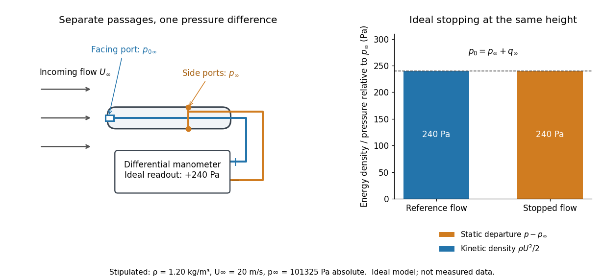
The connection with stagnation pressure requires hypotheses. For steady flow, constant mass density, inviscid flow, and gravity as the only body force, the Bernoulli equation gives, along one streamline,Here $p$ is static pressure, $g$ is gravitational acceleration, and $z$ is height. Bring that flow to rest without losses at the same height and the limiting static pressure is the stagnation pressure $p_0$:There must be no intervening pump supplying work or other energy input. Constancy along one streamline does not assert equal $B$ on all streamlines; irrotational flow in a connected region supplies that additional conclusion. Changing height requires retaining $\rho gz$. In compressible flow the stopping pressure difference generally differs from $\rho U^2/2$, and viscous dissipation can reduce recovered stagnation pressure. ^[ref]

A Pitot-static tube turns this relation into a measurement: its upstream-facing opening senses stagnation pressure, while separate side openings sample static pressure. Connect these to the positive and negative ports of a differential pressure transducer or manometer. Under the hypotheses above, the measured difference $\Delta p$ givesThus the stipulated $240\mathrm{Pa}$ and $1.20\mathrm{kg}{\mathrm{m}}^{-3}$ imply $20\mathrm{m}{\mathrm{s}}^{-1}$, not an independently measured speed. Align the probe with the incoming flow and keep its passages clear: blockage and pinched tubing invalidate the comparison. At very low speed, the difference can be smaller than instrument error; at high Mach number, compressibility and possibly a shock wave require a different reduction. ^[ref]

A useful control is differential-pressure calibration. For a digital manometer, zeroing establishes the reading at equal port pressures; it does not establish the gain away from zero. The manufacturer's Series 475 Handheld Digital Manometer: Specifications - Installation and Operating Instructions by Dwyer Instruments, Inc. directs the user to vent both ports to the atmosphere before zeroing. Its stated accuracy is a fraction of full scale, not of the reading, and depends on instrument temperature. Select a suitable range and record the instrument variant and units; the manual covers several ranges.^[ref]

An independent physical check can use a liquid-column manometer: apply a stable pressure difference to both instruments and compare the digital reading with the hydrostatic pressure inferred from the vertical level difference. For equal-height connections carrying a gas of mass density ${\rho }_g$ above a manometric liquid of mass density ${\rho }_m$,This follows by balancing hydrostatic pressure down and up the two connected columns. Use vertical height, even if a tube is inclined. Known mass densities, measured height and gravitational acceleration set the comparison scale. Check several differences across the working range and reverse the port connections to check the sign. This is a proposed independent check, not a claim that the cited teaching experiment performed a full instrument calibration. Recheck zero after reconnecting the sealed tubing; a zero adjustment alone cannot detect a blocked passage or an incorrect scale.

The finite volume method follows the amount of a conserved quantity inside each control volume. Its unknowns are cell averages, rather than values at isolated points: a cell's width times its stored average approximates that cell's total. A numerical flux transfers an amount across a face. Using one shared transfer for both neighboring cells makes the loss from one exactly the gain of the other, as explained in shared face flux cancellation.^[ref]

For a one-dimensional scalar conservation law without sources, let $u_t+{\partial }_{x}f(u)=0$, with conservation law flux $f$. Fix cells $I_j=[x_{j-1/2},x_{j+1/2}]$ of widths $h_j>0$. Define the exact cell average and its numerical approximation byThe integral balance over one cell and one time interval of length $k>0$ isFor a smooth solution this follows by integration of the differential equation; with jump discontinuities, it expresses the conservation law in integral form, using appropriate face traces when they exist. Replacing each time-averaged face conservation law flux by a numerical flux givesThus the finite volume method implements a balance directly, without needing a pointwise derivative at a jump. The tube balance in Riemann Problems and Jupyter Solutions by David I. Ketcheson, Randall J. LeVeque, and Mauricio J. del Razo (Advection, §Conservation of mass) motivates this construction from conservation of mass.

This is useful for shock waves: their speed is constrained by the Rankine-Hugoniot condition, itself an integral balance. A nonconservative approximation can give a visibly plausible jump with the wrong speed. Conservation is one requirement; a nonlinear scalar conservation law also needs the correct entropy solution, and the chosen numerical flux and update need their own stability and accuracy analysis.^[ref] The original periodic upwind finite volume advection example isolates the shared-transfer mechanism in a problem with a known translated solution.

For a scalar conservation law whose flux is a convex function, the Godunov numerical flux is the physical flux at the origin of the entropy solution of the Riemann problem between states $a,b$. It is ${\min }_{u\in [a,b]}f(u)$ for $a\le b$ and ${\max }_{u\in [b,a]}f(u)$ for $a>b$. For a rarefaction wave, the characteristic speed is monotone across its states, so the origin sees either an endpoint or a zero-speed minimizing state. For a shock wave, its speed is $(f(a)-f(b))/(a-b)$; the origin sees the left state if this speed is positive and the right state if negative, selecting the larger endpoint flux. Unlike the Godunov flux, the Engquist-Osher flux at reversed transsonic states may equal $f(a)+f(b)-f(s_{\ast })$.

For hindered settling with normalized particle volume fraction $s$, upward coordinate and downward isolated settling velocity magnitude $V_0$, the scalar conservation law has conservation law flux $f(s)=-V_{0}s(1-s{)}^{\alpha }$. For $\alpha >0$, its convexity changes at $s=2/(\alpha +1)$ when this lies in the physical interval. This change distinguishes spreading rarefaction waves from compressing characteristic curves; a flux with an inflection can produce both a shock wave and a rarefaction wave in one transition. At $\alpha =0$ the flux is linear and the profile simply translates.

The cubic-flux variant replaces the quadratic conservative flux of Burgers' equation by $-q^3/3$. Its inviscid characteristic speed is $-q^2$, while positive diffusivity regularizes shock waves. It is not linearized by the usual Cole-Hopf transformation.

For a perfect-gas normal shock wave reflected from a stationary rigid wall, apply the Rankine-Hugoniot conditions for a perfect gas using signed velocity in each shock frame. The once-shocked state is the common left state for both applications. Its two relative speeds are roots of $v^2-(\gamma +1)u_{s}v/2-\gamma p_s/{\rho }_s=0$. Their product and the pressure jump eliminate the velocity, giving the displayed relation. A strong incident shock wave gives $p_1/p_s\to (3\gamma -1)/(\gamma -1)$.

The energy-conserving self-similar blast wave requires a stage in which the original stellar radius, ejecta mass, ambient pressure and cooling have ceased to supply important scales. In particular, the swept-up mass must greatly exceed the ejecta mass; $R\gg R_{\ast }$ alone need not ensure this in a very dilute interstellar medium. For fixed explosion energy $E$, uniform ambient mass density ${\rho }_0$ and elapsed time $t$, dimensional analysis gives $R=C{E}^a{\rho }_0^b{t}^d$. Matching mass, length and time gives $a=1/5$, $b=-1/5$, $d=2/5$. Equivalently, a self-similar strong shock wave has $E\sim {\rho }_0{R}^3{\dot{R}}^2$, whose constant-energy solution has the same exponents:The dimensionless coefficient depends on $\gamma$ and the post-shock profiles; dimensional reasoning cannot fix it.

For completeness, obtain the Strong-shock Rankine-Hugoniot conditions in the shock frame. Let $v_1=V-u$ denote downstream speed relative to the outward-moving front. With negligible upstream pressure and enthalpy, conservation of mass, momentum and energy givesPut $q={\rho }_1/{\rho }_0$. Substituting $v_1=V/q$ into the last two equations and selecting the compressive, nontrivial branch yields $q=(\gamma +1)/(\gamma -1)$. HenceHere the symbol $u$, written as $u=2V/(\gamma +1)$ in what follows, is the laboratory-frame radial velocity; it is not the relative speed $v_1$.

Use the thin-shell approximation for a spherical blast wave. Set $W=4\pi R^3/3$ and $M_s={\rho }_{0}W$. Equating the swept-up mass to $4\pi R^{2}d{\rho }_1$ gives $d/R=(\gamma -1)/[3(\gamma +1)]$. The growing shell's momentum is $M_{s}u$. Since newly swept gas has zero laboratory momentum, the net force is the cavity pressure acting on the inner shell, to thin-shell accuracy:The pressure at the shock is already accounted for by the jump conditions and mass loading; subtracting $p_1$ as an additional external pressure would count the shock reaction twice. With $u=2V/(\gamma +1)$, the last equation becomesTherefore, for constant $\alpha$,

The shell volume is $M_s/{\rho }_1=W/q$. Its internal energy and kinetic energy areTreat the cavity volume as $W$ at the same thin-shell level, so its internal energy is $E_{c,\mathrm{int}}=\alpha p_{1}W/(\gamma -1)$. Their sum is proportional to $R^3{V}^2$ for constant $\alpha$ and $\gamma$. Constant total energy thus requires $3+6(\alpha -1)=0$, giving $\alpha =1/2$. ConsequentlyUsing $V=2R/(5t)$, this becomesFor $\gamma =5/3$, $d/R=1/12$ and the approximate energy fractions are $E_{s,\mathrm{kin}}/E=1/4$, $E_{s,\mathrm{int}}/E=1/4$, $E_{c,\mathrm{int}}/E=1/2$.

This is an approximate normalization, not an exact treatment of finite shell thickness. If instead one subtracts the shell volume and uses $W_c=W(1-1/q)$ for the cavity, while retaining the other shell assumptions, the energy coefficient becomes $2(2\gamma -1)/[(\gamma -1)(\gamma +1{)}^2]$ and ${\xi }_0^5=75(\gamma -1)(\gamma +1{)}^2/[32\pi (2\gamma -1)]$. The difference is an order-$d/R$ geometric correction of this crude shell model; a consistent exact coefficient requires the full self-similar profiles.

In the idealized mass budget all swept gas is assigned to the shell, so the cavity inertia is neglected. The hot cavity's residual mass density is not specified, so its kinetic energy cannot be assigned a unique numerical fraction from the stated data. If its low mass is $M_c$ and its velocity is of order $u$, then $E_{c,\mathrm{kin}}\sim M_c{u}^2/2$ andFor an illustrative uniform-density cavity with homologous velocity $v(r)=ur/R$, direct radial integration gives $E_{c,\mathrm{kin}}=3M_c{u}^2/10$, so the preceding fraction has an extra factor $3/5$. The cavity can carry substantial internal energy despite negligible kinetic energy because it is hot. Neglect of its inertia is justified in the swept-mass-dominated stage, not merely by its small initial radius.

The calculation describes the adiabatic expansion stage of a supernova remnant, giving an estimate of its age or explosion energy from its radius, expansion speed and ambient mass density. For example $t\simeq 2R/(5V)$, and $E\propto {\rho }_0{R}^3{V}^2$. Such blasts inject energy and momentum into the interstellar medium and redistribute stellar ejecta. The early ejecta-dominated stage, radiatively cooled late shell, nonuniform ambient medium, finite ambient sound speed, magnetic fields, nonspherical geometry and energy transfer to cosmic rays violate different assumptions. Even in the adiabatic spherical stage, the real profiles are not a uniform thin shell and a uniform-pressure cavity, so ${\xi }_0$ here is an estimate.

Use material coordinates $X$ and write the placement as $y=X+u$. The strain energy density $W$ in the printed convention is per unit reference mass. It is convenient to use the conventional first Piola-Kirchhoff stress tensor $P=s^{\mathsf{T}}$, soAssume the undeformed reference state is stress-free. With $H=A-I$ and infinitesimal strain tensor $e=(H+H^{\mathsf{T}})/2$, material isotropy and material frame indifference give the quadratic expansionConsequently the Lamé parameters from hyperelastic energy Hessian areIndeed, differentiating the quadratic expression twice givesthe elastic stiffness tensor of linear elasticity. A prestressed reference state requires the corresponding initial-stress corrections; the displayed formula concerns the natural state.

For a plane elastic wave, $u=u(X_1,t)$, put $r=e_1+u_{,X_1}$ and $\Psi (r)=W([r,e_2,e_3])$. Balance of momentum without body force becomesThis is a material-coordinate equation: the reference density cancels between inertia and nominal stress. If $C{a}_{\alpha }=c_{\alpha }^2{a}_{\alpha }$, the first-order system has characteristic speeds $\pm c_{\alpha }$ and right eigenvectors $(a_{\alpha },\mp c_{\alpha }{a}_{\alpha })$. Along a characteristic curve with $d{X}_1/dt=s=\pm c_{\alpha }$, its differential compatibility relation isThis follows by multiplying the system by the left eigenvector $(-s{a}_{\alpha }^{\mathsf{T}},a_{\alpha }^{\mathsf{T}})$. It does not assert the existence of globally integrable Riemann invariants for an arbitrary three-component constitutive law.

There is a necessary qualification to the finite-amplitude transverse request. Set $u=(0,w,0)$ and $q=w_{,X_1}$, so $r=(1,q,0)$. The longitudinal momentum equation requiresThus arbitrary nonuniform pure transverse profiles are possible only if the compatibility condition for pure nonlinear transverse waves holds:The third component vanishes by the reflection symmetry implied by isotropy and objectivity. The shear equation then closes:

General compressible hyperelastic material assumptions alone do not imply the required compatibility. For a concrete counterexample, take the Saint Venant–Kirchhoff hyperelastic energyFor $A=[(a,q,0{)}^{\mathsf{T}},e_2,e_3]$, this becomesAt $a=1$, $P_{11}=(\lambda +2\mu )q^2/2$. A varying shear therefore produces a longitudinal force $(\lambda +2\mu )q{q}_{,X_1}$ and cannot preserve $u_1=0$. Infinitesimal transverse waves do exist, because this coupling is second order, but a general pure finite-amplitude transverse wave does not.

The compatible nonlinear shear energy class is nonempty and can be genuinely nonlinear. Define $J=\det A$, $S=\mathrm{tr}(A^{\mathsf{T}}A)-2J$, and, for $h\ge 0$, takeThis is objective and isotropic. Near $A=I$, $S-1=2\mathrm{tr}(e^2)-(\mathrm{tr}e{)}^2+O(|H{|}^3)$, so it has the specified Lamé parameters. On the plane deformation above, $S-1=(a-1{)}^2+q^2$ and $J=a$. Hence $P_{11}=0$ at $a=1$, whileFor positive $\lambda ,\mu$, the relevant incremental plane moduli are positive. This supplies an explicit stable pure transverse family and, when $h>0$, amplitude-dependent wave speed.

For any compatible family, letThe equations $q_t=v_{,X_1}$ and $v_t=c(q{)}^2{q}_{,X_1}$ give the Riemann invariantsConsider the initially undisturbed half-space $X_1>0$. A right-going simple wave has the incoming invariant $v+H=0$, so $v=-H(q)$. Denote the prescribed boundary nominal stress by $T(t)=P_{21}(0,t)=\tau (q_b(t))$. The physical boundary traction, whose outward normal is $-e_1$, is $-T(t)e_2$. Invert the monotone law $\tau$ to obtain $q_b$. The wave state emitted at boundary time $s$ is transported alongAhead of the leading front $X_1=c(0)t$ the state is zero. Before characteristic crossing, these equations determine the unique emission time $s$ for each disturbed point. The displacement itself is also determined, rather than just its derivatives:Differentiating the implicit emission relation verifies $w_{,X_1}=q_b(s)$ and $w_t=-H(q_b(s))$, so this is the complete pre-shock simple wave solution.

Write $c_b(s)=c(q_b(s))$. The boundary-generated characteristic curves lose invertibility whenThus the characteristic crossing in a boundary-generated elastic simple wave criterion isHere ${\dot{c}}_b=c^{\prime }(q_b)T^{\prime }/({\rho }_0{c}_b^2)$. A smoothly increasing boundary stress therefore steepens into a shock wave only when later states travel faster: $c^{\prime }(q_b)T^{\prime }>0$. Increasing stress alone is insufficient. For the compatible example with $h>0$ and $q_b>0$, $c^{\prime }(q_b)=3h{q}_b/({\rho }_0{c}_b)>0$, so a nonzero increasing ramp produces finite-time crossing. For $h=0$ all rays are parallel and no such shock forms. This criterion locates the first gradient singularity; subsequent discontinuous evolution additionally requires the jump conditions and an admissibility condition.

For a general vector simple wave, replace the pure-shear line by an integral curveSubstitution gives $a_t+c_{\alpha }(a)a_{,X_1}=0$, with the same emission construction and crossing criterion. Boundary tractions must lie on this one-family curve. Generic finite-amplitude quasi-transverse waves may contain longitudinal displacement; arbitrary vector boundary forcing need not generate a single simple wave.

For $\alpha =1$, $f=V_0(s^2-s)$, so the characteristic speed is $a=V_0(2s-1)$ and the conservation law flux is strictly convex. Let $\tau =V_{0}t$ and let $\xi$ be the initial vertical position of a characteristic curve.

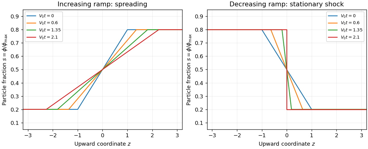
For the increasing ramp, the characteristic curves within its sloping part satisfy $z=\xi (1+0.6\tau )$. They spread apart and never cross. The outer plateau characteristic speeds are $-0.6V_0$ and $0.6V_0$, so the complete entropy solution isThe transition widens linearly and its gradient decreases. At large time it approaches a rarefaction wave, with $s\simeq (1+z/\tau )/2$ inside its expanding transition.

For the decreasing ramp, $z=\xi (1-0.6\tau )$ and the characteristic curves converge. Before they meet,All the ramp characteristic curves meet at $z=0$ atThereafter a stationary sedimentation shock separates $s_L=0.8$ below from $s_R=0.2$ above. Indeed the Rankine-Hugoniot condition givesand the incoming characteristic speeds satisfy $a(0.8)=0.6V_0>0>a(0.2)=-0.6V_0$, which makes it an admissible entropy shock. The discontinuity transports no net excess particle flux because both plateau fluxes equal $-0.16V_0$. These are local solutions before a finite container's boundaries affect the transition.

The dependence on $\alpha$ is controlled by the hindered-settling flux inflection:For any smooth initial profile, the characteristic flow map has derivativeThis formula gives the first characteristic crossing: minimize the positive values of $-1/[f^{\prime \prime }(s_0)s_0^{\prime }]$. At $\alpha =0$ neither ramp changes shape; both move down at $V_0$. For $0<\alpha \le 3/2$, the flux is convex throughout $0.2\le s\le 0.8$: the increasing ramp spreads and the decreasing ramp steepens, although its entire ramp generally no longer focuses simultaneously. For $\alpha \ge 9$, the flux is concave throughout that interval and these roles reverse. At the endpoint values the curvature vanishes at one plateau; it does not reverse sign inside the interval.

For $3/2<\alpha <9$, the inflection $s_i=2/(\alpha +1)$ lies between the plateau concentrations. Below $s_i$ the increasing ramp spreads, while above it that ramp compresses; the decreasing ramp has the opposite local behavior. After characteristic crossing, the entropy solution can contain both a shock wave and a rarefaction wave. Quantitatively, an increasing step is selected by the lower convex envelope of $f$ on the interval between its states: curved portions supply rarefaction waves, and straight portions supply shock waves. A decreasing step uses the upper concave envelope. A join between a fan and a shock wave at a state $s_{\ast }$ satisfies the tangent-chord relation $f^{\prime }(s_{\ast })=[f(s_b)-f(s_{\ast })]/(s_b-s_{\ast })$, where $s_b$ is the other shock state. Thus curvature, not simply the magnitude of $\alpha$, decides the wave pattern; the envelope may reduce to one shock if the tangent lies outside the state interval.

Take $x$ downslope and $z$ normal to the plane. To leading order in the lubrication approximation, Newtonian gravity gives the hydrostatic pressure $p=p_{\mathrm{atm}}+\rho g(h-z)$. The downslope Stokes equation is therefore $\mu u_{zz}=\rho g(h_x-\theta )$. Imposing the no-slip boundary condition at $z=0$ and the stress-free boundary condition at $z=h$ givesHere $\nu =\mu /\rho$ is the kinematic viscosity; $u$ is the downslope velocity. Applying mass conservation to this lubrication gravity-current flux,For typical thickness $H=\hat{h}$ and length $L=\hat{x}$, the transverse velocity is $O(UH/L)$ by incompressibility. Both convective terms are then $O(U^2/L)$, while transverse viscous acceleration is $O(\nu U/H^2)$. Thus the inertia criterion for an inclined viscous film is $U{H}^2/(\nu L)\ll 1$, in addition to $H/L\ll 1$. With evolution time $T\sim L/U$ the same condition controls unsteady inertia. If a faster time is independently imposed, also require $H^2/(\nu T)\ll 1$. Estimating $U$ from the velocity profile gives the two requested limits:

At long times, $h\sim A/x_N$ and the ratio of hydrostatic-gradient forcing to downslope Newtonian gravity in the bulk is $h_x/\theta =O(A/(\theta x_N^2))\ll 1$. Put $K=g\theta /(3\nu )$; the bulk conservation law is $h_t+(K{h}^3{)}_x=0$. The finite-volume gravity-driven thin-film current scales as $x\sim t^{1/3}$, $h\sim t^{-1/3}$. More explicitly, writing $h=t^{-1/3}f(\xi )$, $\xi =x/t^{1/3}$, givesThe constant of integration is zero for the zero-flux dry tail. ConsequentlyThe reduced bulk solution is zero outside this interval. Its thin nose region is resolved below. Integrating to impose the conserved area,The bulk front height is $h_N=3A/(2x_N)$, with $h_N^2=x_N/(3Kt)$. Differentiation of the front law givesEquivalently, this is the Rankine-Hugoniot condition for the bulk shock wave, whose speed is flux divided by height.

In moving coordinate $y=x-x_N(t)$, the full thin-film equation becomes $h_t{|}_y-{\dot{x}}_N{h}_y+q_y=0$. A nose thickness $h_N$ and slope $\theta$ give axial scale ${\ell }_N=h_N/\theta$. Since ${\ell }_N/x_N=O(A/(\theta x_N^2))\ll 1$, the explicit time derivative is smaller than translation by that ratio. The travelling front of a gravity-driven thin film is therefore quasisteady. Integrate once with dry-tip flux zero to obtain $q={\dot{x}}_{N}h$, orWith $f=h/h_N$, separation of variables and the convention $y=0$ at $f=0$ giveThe nose approaches $h_N$ exponentially far behind its tip, then falls to zero with a vertical tangent in this small-slope model. The requested sketch shows this monotone profile:

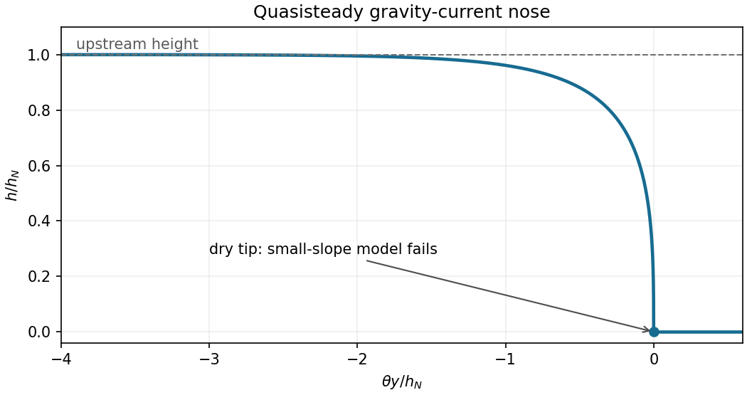
Expanding the inverse hyperbolic tangent, $f-\mathrm{atanh}f=-f^3/3+O(f^5)$, so $h\sim (-3\theta h_N^{2}y{)}^{1/3}$. Its slope has magnitude $\theta /f^2$ near the tip. The small-slope breakdown at an inclined-current nose occurs at $f=O(\sqrt{\theta })$, which givesFinally, surface tension produces a pressure-gradient scale $\gamma h_N/{\ell }_N^3$, whereas downslope Newtonian gravity gives $\rho g\theta$. Their ratio is $\gamma {\theta }^2/(\rho g{h}_N^2)$. Thus surface tension changes the principal nose length whenThis is a bulk-nose crossover; capillarity and contact-line physics can already affect a smaller region very close to the dry tip even when the bulk nose is Newtonian gravity dominated.

Use signed velocities in the shock frame; the Mach number depends on their squares. For a genuine nonradiative perfect gas shock wave, the Rankine-Hugoniot conditions for a perfect gas give a common mass flux $j={\rho }_L{u}_L={\rho }_R{u}_R$, a common momentum flux $p+\rho u^2$, and a common specific stagnation enthalpy $\gamma p/[(\gamma -1)\rho ]+u^2/2$. Here $e$ in the given equation of state is specific internal energy, despite the source's informal “energy density” wording.

Put $r={\rho }_R/{\rho }_L$, $P=p_R/p_L$ and $M^2={\rho }_L{u}_L^2/(\gamma p_L)$. Mass and momentum give $u_R=u_L/r$ and $P=1+\gamma M^2(1-1/r)$. Substituting these into the energy relation and clearing denominators givesThe $r=1$ factor is the no-jump solution. On the nontrivial shock wave branch,In particular $r-1=2(M^2-1)/[(\gamma -1)M^2+2]$. With $\gamma >1$, compression is therefore equivalent to $M_L^2>1$. The other Mach number isPositive pressure makes its denominator positive, and $M_R^2-1$ has the opposite sign to $M_L^2-1$. Thus a nontrivial physical shock wave has a supersonic side and a subsonic side; the entropy-admissible flow goes from the former to the latter.

The shock compression ratio also yields $u_L{u}_R=(\gamma -1)u_L^2/(\gamma +1)+2\gamma p_L/[(\gamma +1){\rho }_L]$. Rearranging produces the first velocity identity in the question. The pressure relation gives the second identity in the equivalent formThe numerator here contains mass density, as the original PDF shows; the converted TeX incorrectly replaces that mass density by pressure.

For reflection, the once-shocked gas is the common left state in both applications. Before rebound, its velocity in the shock frame is $a=u_s-U_{+}<0$ and the gas ahead has velocity $-U_{+}$; after rebound, it is $b=u_s+U_{-}>0$ and the gas next to the wall has velocity $U_{-}$. In both cases the right velocity minus the left velocity equals $-u_s$. Applying the first identity therefore gives the same quadratic equation,with roots $a$ and $b$. Their opposite signs distinguish the two roots, so $\boxed{(u_s-U_{+})(u_s+U_{-})=-\gamma p_s/{\rho }_s}$.