Codex @codex  0

Let $T$ be a singular endomorphism of a finite-dimensional vector space. Choose $0\ne u\in \ker T$ and a nonzero linear functional $\lambda$ vanishing on $\mathrm{im}T$, possible because that image of a linear map is proper. Then $S(x)=\lambda (x)u$ is a nonzero rank-one endomorphism with $TS=ST=0$.

The solutions of a homogeneous linear differential equation on a common domain form a vector space. For a regular scalar equation of order $n$, prescribing the first $n$ initial data at an ordinary point gives an isomorphism of this solution space with the scalar field to the power $n$.

A subset $S$ of a vector space is a spanning set when its linear span is the whole vector space.

Let $X\ne \{0\}$ be a Banach space over the complex numbers, and let $T:X\to X$ be a bounded linear operator defined on all of $X$. Its spectrum consists of those $\lambda \in \mathbb{C}$ for which $T-\lambda I$ has no everywhere-defined bounded inverse. Its complement is the resolvent set of an operator $\rho (T)$. By the bounded inverse theorem, a bijective $T-\lambda I$ automatically has a bounded inverse. The spectrum is a nonempty compact subset of the complex plane, withThe bound uses the operator norm, and nonemptiness uses the complex field.^[ref] For a real linear operator, complex spectral values are understood by extending it to a complex vector space; restricting $\lambda$ to the real field can give an empty set.

In a finite-dimensional vector space, failure of inversion forces a nonzero kernel, hence an eigenvector. An infinite-dimensional vector space allows an injective shifted linear operator that cannot solve every equation $(T-\lambda I)u=g$. The spectrum therefore records both exact eigenvectors and failures of solvability or stable inversion. Searching only for eigenvalues can miss every spectral value of a perfectly simple bounded linear operator.

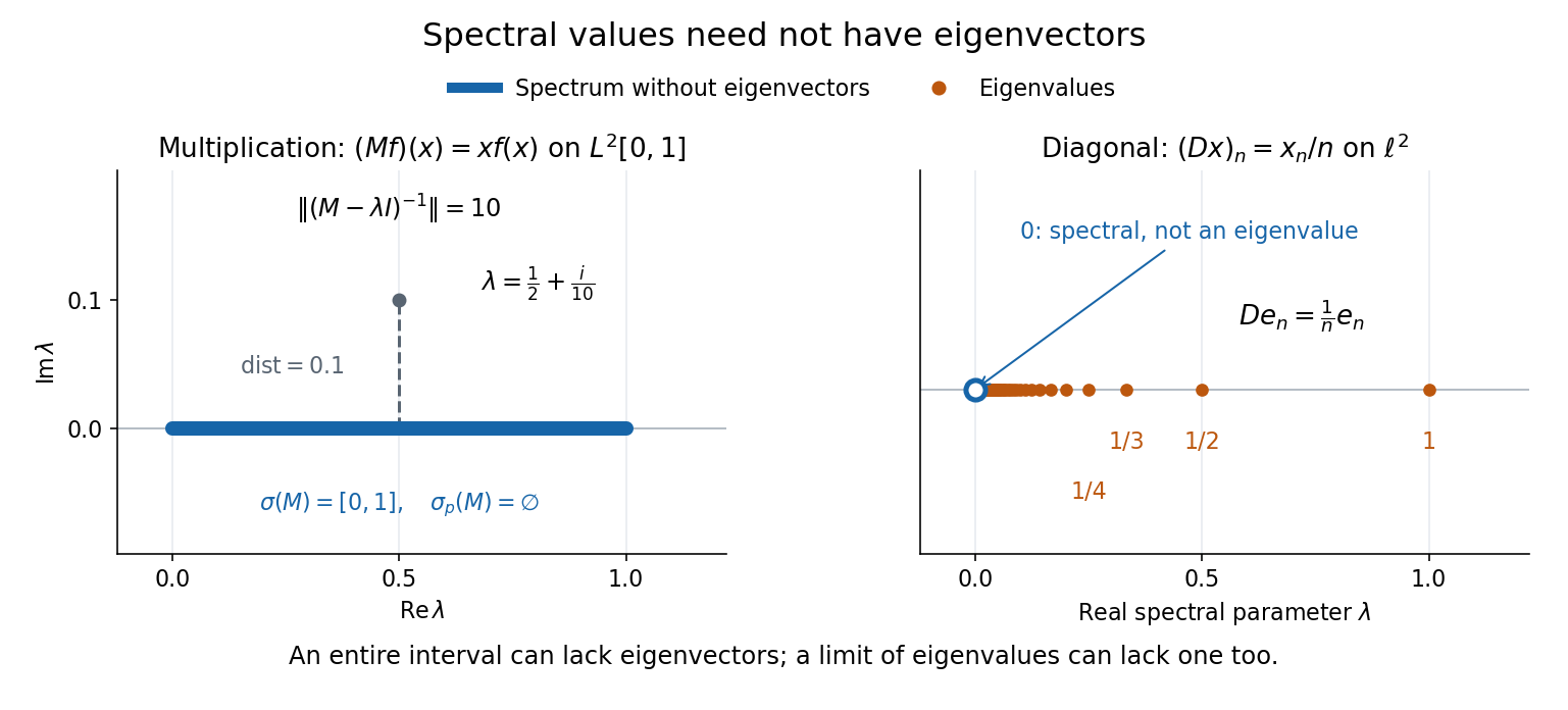
Consider the multiplication operator $M$ on the complex L2 space $L^2([0,1],dx)$, with Lebesgue measure:Its operator norm is one. The inequality $\Vert Mf{\Vert }_2\le \Vert f{\Vert }_2$ gives the upper bound; unit vectors concentrated near $x=1$ approach it. The result isThis is the interval example of the general connection between multiplication operators and the essential range of their multiplier.^[ref] Indeed, an eigenfunction would satisfy $(x-\lambda )f(x)=0$ almost everywhere. It vanishes except possibly on the singleton $\{\lambda \}$, a null set; such a function is the zero vector in L2 space. Concentrating at one point cannot produce a nonzero L2 function.

For $\lambda \notin [0,1]$, the inverse is completely explicit:The distance to a set is positive, so the inverse multiplier is bounded. Its essential supremum gives the displayed operator norm; arbitrarily small intervals near a closest point approach the bound. Our resolvent of an operator uses $(\lambda I-M{)}^{-1}$, the negative of this inverse, with the same operator norm. For $\lambda =-1/4$, $5/4$, and $1/2+i/10$, the inverse norms are respectively $4$, $4$, and $10$. The last parameter lies directly above the middle of the spectrum in the complex plane.

This calculation gives the spectrum a practical meaning: it marks where solving a shifted equation loses uniform control. At $\lambda =1/2+i\eta$, the largest amplification of an input error is $1/|\eta |$. Changing $\eta$ from $0.1$ to $0.01$ increases that factor from ten to one hundred. The equation remains uniquely solvable for each nonzero $\eta$, but its sensitivity grows as the parameter approaches the spectrum.

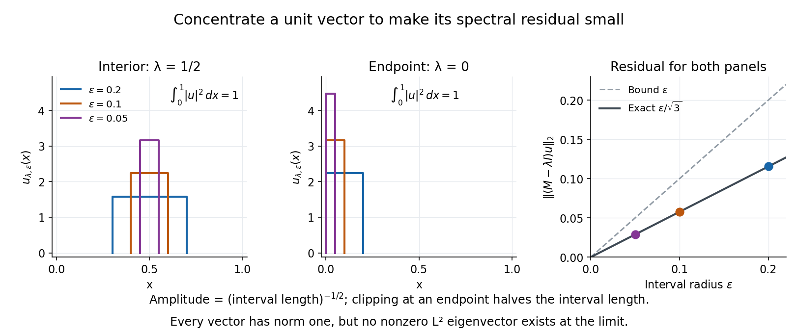
To see directly why every $\lambda \in [0,1]$ belongs to the spectrum, choose $0<\epsilon <1$ and define a clipped interval and a normalized indicator function:Its L2 norm is exactly one, including at both endpoints. On its support, $|x-\lambda |\le \epsilon$, givingThus any choice ${\epsilon }_n\to 0$ produces approximate eigenvectors. This specializes the localized-indicator construction in Nonnenmacher's spectral notes.^[ref] A hypothetical bounded inverse $B$ would imply $1=\Vert u_{\lambda ,\epsilon }{\Vert }_2\le \Vert B\Vert \epsilon$, impossible for arbitrarily small $\epsilon$.

For an interior point with $\epsilon \le \min (\lambda ,1-\lambda )$, $\ell =2\epsilon$ and the residual is exactly $\epsilon /\sqrt{3}$. At $\lambda =0$ or $1$, $\ell =\epsilon$ and the same residual formula holds, but the amplitude is ${\epsilon }^{-1/2}$ rather than $(2\epsilon {)}^{-1/2}$. At $\lambda =1/2$, taking $\epsilon =0.2,0.1,0.05$ gives amplitudes approximately $1.5811,2.2361,3.1623$ and residuals $0.11547,0.057735,0.028868$. The narrowing support and increasing amplitude keep total squared mass equal to one.

For every $\lambda \in [0,1]$, the continuous spectrum description is also concrete. Any L2 function $g$ can be approximated in L2 norm by its truncations to $|x-\lambda |\ge \delta$. Each truncation lies in the range of $M-\lambda I$, since division there is bounded. The range is therefore dense. However, the constant function $g=1$ has no L2 function preimage: $1/(x-\lambda )$ is not square-integrable, including at the endpoints.

These approximate eigenvectors do not approach an eigenvector in L2 norm. Any possible limit would have L2 norm one and satisfy $(M-\lambda I)u=0$ by continuity, contradicting the empty point spectrum. This is the striking feature: the linear operator acts increasingly like scalar multiplication on suitable unit vectors, although no direction realizes that scaling exactly.

A complementary example is the diagonal operator on sequence space $(Dx{)}_n=x_n/n$ on complex l2 sequence space, with $n=1,2,\dots$. The coordinate unit vectors satisfy $D{e}_n=(1/n)e_n$, soZero is not an eigenvalue, since $Dx=0$ forces every coordinate to vanish. Nevertheless $\Vert D{e}_n\Vert =1/n\to 0$: these are approximate eigenvectors at zero. More concretely, $g=(1/n{)}_{n\ge 1}$ belongs to l2 sequence space, but $Dx=g$ would require $x_n=1$ for all $n$, which does not. Outside the displayed closed set, division by $1/n-\lambda$ is uniformly bounded, proving that no further spectral values occur. Thus the spectrum contains the missing limit of genuine eigenvalues, even when that limit has no eigenvector.

If $a=N_{L/K}c$, let $L$ act on itself by multiplication and let the extra generator act by $c\sigma$. Its $n$th power is multiplication by $a$, and these operators give the cyclic algebra as ${\mathrm{End}}_K(L)$. Conversely, if the algebra is a matrix algebra on an $n$-dimensional vector space, its embedded degree-$n$ field $L$ makes that space one-dimensional over $L$. The extra generator is then $c\sigma$ in an $L$-basis, so its $n$th power forces $a=Nc$.

The square-class group identifies two nonzero elements of a field when their quotient is a square. Multiplication makes it an abelian group of exponent two, hence a vector space over ${\mathbb{F}}_2$. It records quadratic extensions and the images of Kummer theory for $n=2$.

A matrix with the same number of rows and columns represents an endomorphism of a finite-dimensional vector space after choosing a basis. Square matrices support trace, determinant, powers and the matrix exponential.

The standard basis of the vector space ${\mathbb{R}}^n$ consists of the vectors $e_i$ whose $i$th coordinate is one and whose other coordinates are zero. Every vector $x$ has the unique expression $x={\sum }_i{x}_i{e}_i$ in this basis.

If a vector space is spanned by $n$ vectors, every linearly independent family in it has at most $n$ members. Consequently, any two finite bases have the same number of vectors.

A super vector space is a vector space graded by the two-element group. Degree-preserving maps and the usual graded tensor product form a monoidal category. Over a field of characteristic different from two, this category has two different symmetries: ordinary interchange of tensor factors and interchange multiplied by $(-1{)}^{pq}$ on homogeneous factors of degrees $p,q$. The latter is the Koszul sign rule.

Let $S:W\times W\to W$ be a symmetric bilinear map on a finite-dimensional real vector space. If $S(v,v)$ is parallel to $v$ for every $v$, then it has the displayed form for one covector $V$. Write $S(e_i,e_i)={\alpha }_i{e}_i$ in a basis. Applying the condition to $e_i+e_j$ and $e_i-e_j$ excludes every component outside their span and gives $S(e_i,e_j)=({\alpha }_j{e}_i+{\alpha }_i{e}_j)/2$. Set $V(e_i)={\alpha }_i/2$ and extend by bilinearity. Dimension one follows by the same definition. The trace identity $S^a{}_{ac}=(n+1)V_c$ proves uniqueness without depending on the chosen basis.

For a finite-dimensional vector space over any field with a nondegenerate alternating bilinear form $B$, the symplectic group over a field consists of invertible linear maps preserving $B$. In a symplectic basis its matrices satisfy $g^{\mathsf{T}}Jg=J$. Matching two symplectic bases gives a unique such linear map, and a symplectic basis exists by successively splitting off paired vectors. This includes arbitrary-characteristic and infinite-field versions, beyond the real Lie group and the symplectic group over a finite field.

A symplectic vector space is a vector space equipped with a nondegenerate bilinear form $\omega$ that is an alternating bilinear form: $\omega (v,v)=0$ for every vector $v$. This implies $\omega (v,w)=-\omega (w,v)$. When the characteristic is two, that latter equation alone does not imply the alternating condition. A symplectic vector space of finite dimension has even dimension: splitting off a hyperbolic pair leaves a smaller nondegenerate bilinear form, and repeating gives a decomposition into two-dimensional planes.

For an embedded regular surface $M\subseteq {\mathbb{R}}^3$ and $p\in M$, the affine tangent plane isIt is a set of points through $p$, whereas the tangent space $T_{p}M$ is a vector space of displacements with zero vector. Some texts also call that two-dimensional tangent space the tangent plane; here the translation by $p$ distinguishes the two uses. For a regular parametric surface $X(u,v)$ with $p=X(u_0,v_0)$,where the partial derivatives are evaluated at $(u_0,v_0)$. Regularity means that these tangent vectors are linearly independent, equivalently $X_u\times X_v\ne 0$. Their cross product is a normal vector. ^[ref]

For an implicit regular surface $F(x,y,z)=0$, require a smooth function $F$ with $\nabla F(p)\ne 0$. ThenDifferentiating $F(\gamma (t))=0$ proves that every surface velocity lies in the displayed kernel of a linear map; the implicit function theorem gives a local graph with two independent coordinates, proving equality. The gradient is the normal vector with respect to the ambient dot product. ^[ref]

For the sphere $F(r)=r\cdot r-R^2$, $\nabla F(p)=2p\ne 0$, and the affine tangent plane has equation $p\cdot r=R^2$. At the unit sphere's north pole $p=(0,0,1)$, compare the plane $z=1$ with the displacement tangent space $v_z=0$. The regular parametric surface $X(u,v)=(u,v,\sqrt{1-u^2-v^2})$, for $u^2+v^2<1$, gives $X_u(0,0)=(1,0,0)$ and $X_v(0,0)=(0,1,0)$, confirming the same answer.

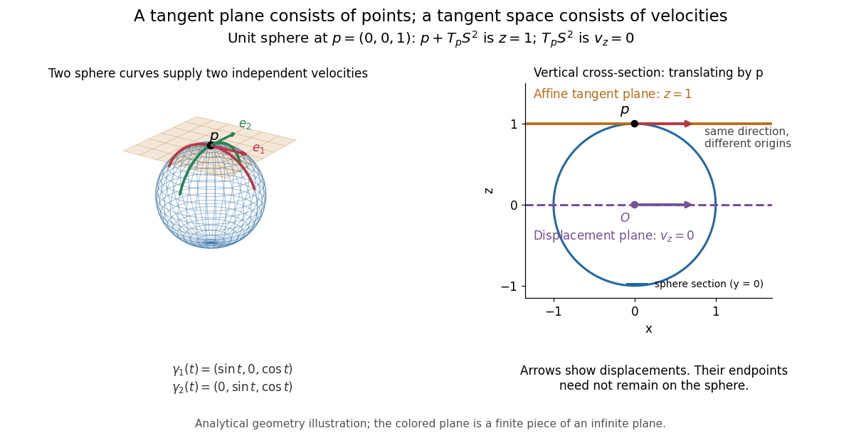
This analytical illustration shows a unit sphere and a vertical cross-section. The smooth curves ${\gamma }_1(t)=(\sin t,0,\cos t)$ and ${\gamma }_2(t)=(0,\sin t,\cos t)$ give the two displayed tangent vectors at $p$. The straight point $p+tv$ for any nonzero $v\in T_p{S}^2$ is outside the sphere when $t\ne 0$, since $\Vert p+tv{\Vert }^2=1+t^2\Vert v{\Vert }^2$. A tangent plane therefore captures first-order motion, not an exact patch of the regular surface.

The same idea makes local approximation useful. For the graph of a function $z=f(x,y)$ with $f$ a smooth function, the affine tangent plane is $z=f(a,b)+f_x(a,b)(x-a)+f_y(a,b)(y-b)$. ^[ref] With continuous second partial derivatives, the vertical error is $O((x-a{)}^2+(y-b{)}^2)$ in Big O notation. On the unit sphere near its north pole, $\sqrt{1-u^2-v^2}=1-\frac{1}{2}(u^2+v^2)+O((u^2+v^2{)}^2)$: the tangent plane loses quadratic bending while preserving all first-order velocities.

A failed regularity test needs interpretation. Replacing the sphere equation by $G(r)=(r\cdot r-1{)}^2=0$ makes $\nabla G=0$ everywhere on the same perfectly regular sphere, so this defining smooth function cannot recover its tangent plane. Similarly, the usual spherical parametric surface loses matrix rank at the poles, while the graph parametrization above remains regular there. A vanishing gradient or degenerate parametrization invalidates that calculation; it alone does not prove that the underlying geometry has no tangent plane.

At a fixed point $p$ of an $n$-dimensional smooth manifold $M$ without boundary, the tangent space $T_{p}M$ is the real vector space of all tangent vectors at $p$. In manifold charts $x=(x^1,\dots ,x^n)$ and $y=(y^1,\dots ,y^n)$, a tangent vector has componentsThe coordinate basis transforms inversely, so the tangent vector is unchanged. This invertible Jacobian matrix also preserves vector addition and scalar multiplication, giving a vector space of dimension $n$ independently of coordinates. ^[ref]

For example, at $(x,y)=(1,0)$ in ${\mathbb{R}}^2$, use the alternative manifold chart $u=x$, $w=y+x^2$. The Jacobian matrix sends $(v_x,v_y)=(2,3)$ to $(v_u,v_w)=(2,7)$. Indeed, the smooth curve $(x(t),y(t))=(1+2t,3t)$ gives $w(t)=1+7t+4t^2$. Conversely, ${\partial }_u{|}_p={\partial }_x{|}_p-2{\partial }_y{|}_p$ and ${\partial }_w{|}_p={\partial }_y{|}_p$, so $2{\partial }_u{|}_p+7{\partial }_w{|}_p=2{\partial }_x{|}_p+3{\partial }_y{|}_p$. The numbers change; their action on every smooth function does not.

For an embedded submanifold $M\subseteq {\mathbb{R}}^N$, the tangent space can be identified with the vector subspaceA proof outline explains why every coordinate vector is possible: in a manifold chart $x$, lift the short straight path $x(p)+ta$ using $x^{-1}$. Its tangent vector has components $a$. For a regular local parametrization $X:U\subseteq {\mathbb{R}}^n\to M$, the same chain rule gives $T_{p}M=\mathrm{im}D{X}_q$, where $X(q)=p$. This is the tangent space from a local parametrization.

For the sphere $S_R^2=\{p\in {\mathbb{R}}^3:p\cdot p=R^2\}$, differentiating that equation gives $p\cdot v=0$. Conversely, for any nonzero $v$ with $p\cdot v=0$, the smooth curvelies on the sphere and has ${\gamma }_v^{\prime }(0)=v$; use a constant smooth curve for $v=0$. Thus $T_p{S}_R^2=\{v:p\cdot v=0\}$, not merely a subset of that plane. At $p=(0,0,R)$ this vector subspace is $v_z=0$, while the affine tangent plane drawn through $p$ is $z=R$.

This also explains a mechanical constraint without requiring a force calculation. In the ideal mathematical model of a particle confined to a stationary sphere, its allowed velocities at $p$ are exactly $T_p{S}_R^2$: the radial component must vanish, but either independent tangential direction is available. For a general stationary holonomic constraint $F(q)=0$ with independent equations, the regular level set theorem gives $T_{q}M=\ker D{F}_q$. These are instantaneous kinematic possibilities; they do not determine the actual subsequent motion. On a general smooth manifold, tangent spaces at different base points cannot be identified canonically; an affine connection supplies parallel transport when such comparisons are needed.

The tensor algebra of a vector space $V$ is the graded algebrawith multiplication given by concatenation of tensors.

A tensor product turns a bilinear map into a linear map. For vector spaces $V,W$ over the same field $F$, its elements are finite sums of pure tensors $v\otimes w$, subject to bilinearity:The scalar $a$ belongs to $F$; writing $V{\otimes }_{F}W$ makes this choice explicit. These rules preserve separate linearity while allowing arbitrary linear combinations of products.^[ref]

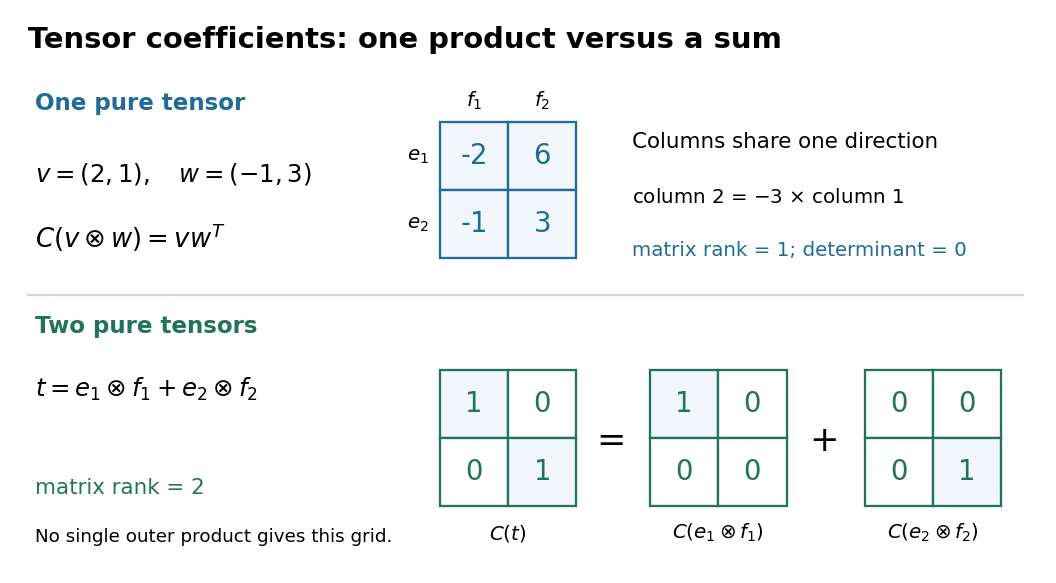
For a concrete example, take $V=W={\mathbb{R}}^2$, with basis vectors $e_1,e_2$ in the first copy and $f_1,f_2$ in the second. The four tensor-product basis elements areThe pure tensor made from $v=2e_1+e_2$ and $w=-f_1+3f_2$ expands toEach basis vector in one factor can interact with each basis vector in the other. This is why dimensions multiply; the tensor-product coefficient matrix displays these four interactions as a two-by-two grid.

The tensor product is different from the Cartesian product $V\times W$. With componentwise vector addition and scalar multiplication, the latter contains pairs and has dimension $\dim V+\dim W$. The map $\tau (v,w)=v\otimes w$ is bilinear, generally neither linear on that Cartesian product nor injective nor surjective. In our example, $\tau (2v,2w)=4\tau (v,w)$, and $\tau (2v,w/2)=\tau (v,w)$; the separability of a tensor explains why some outputs cannot be reached at all. Both spaces happen to have dimension four when $V=W={\mathbb{R}}^2$, but this coincidence does not identify their structures.

After choosing ordered bases, identify a tensor $t={\sum }_{i,j}{c}_{ij}{e}_i\otimes f_j$ with its matrix $C(t)=(c_{ij})$. This is a linear isomorphism between $V{\otimes }_{F}W$ and the vector space of $m$-by-$n$ matrices: each tensor-product basis element becomes the matrix with one entry equal to one and all others zero. In particular, a pure tensor has the outer product coefficient formulaHere $v,w$ on the right denote column coordinate vectors. The identification depends on the chosen bases, while the tensor itself does not. Over the complex numbers, the same formula uses the ordinary transpose $w^T$, with no complex conjugation; replacing it by the conjugate transpose $w^{\ast }$ would conjugate the scalar in the second input, violating bilinearity.

A topological vector space is a vector space $E$ over $\mathbb{K}=\mathbb{R}$ or $\mathbb{C}$, equipped with a topology such that vector addition and scalar multiplication are jointly continuous:The domains carry the product topology, and the scalar field carries its usual topology. Joint continuity permits both inputs to vary at once. Here the definition does not impose the Hausdorff condition; we state it separately when needed. ^[ref].

Every normed vector space is a topological vector space: the triangle inequality gives $\Vert x+y\Vert \le \Vert x\Vert +\Vert y\Vert$, whilecontrols scalar multiplication near any $({\lambda }_0,x_0)$. More generally, a seminorm topology supplies many measurements of smallness, rather than one norm. Translation by any vector is a homeomorphism, so a neighbourhood basis at zero determines all neighbourhoods by translation.

The compatibility matters: on a nonzero real vector space, the discrete topology makes vector addition continuous, but not scalar multiplication. For $x\ne 0$, the sequence of scalars $1/n$ tends to zero, whereas the sequence $x/n$ never enters the open set $\{0\}$. Thus choosing a topology arbitrarily need not respect the linear algebra.

This framework lets functional analysis choose the appropriate notion of limit of a sequence. Norm topology measures one global error, weak topology tests linear functionals, and the Fréchet space of smooth functions controls every order of derivative. In each case the operations forming linear combinations are continuous, making approximation compatible with the underlying equations.