Topics (384k) Articles (398k) Users (410) Discussions (242) Comments (383) Files (13k) New article

Recovery-correction uncertainty quantifies uncertainty in an amount inferred through a recovery correction. If uses measured recovered amount and recovery estimate , both inputs contribute. The uncertainty of the corrected result is not obtained merely by copying the uncertainty attached to .
The first-order sensitivity coefficients are and . Combining them givesThis is the linear propagation of uncertainty law with correlated inputs.[ref]
Evaluation of measurement data — Guide to the expression of uncertainty in measurement by JCGM. §§5.1–5.2, independent and correlated input quantities.
With positive nominal inputs and correlation coefficient , the relative form isRecovery-estimate covariance can matter because an amount and its estimated recovery may share measurements or common response changes.For original values , , and , the corrected amount is . Independence gives relative variance and standard uncertainty about . With , the variance becomes and uncertainty about . Correlation cannot be chosen to improve the answer; it must describe the actual joint measurements.
The formula is an approximation near the nominal values. A recovery near zero or with large relative uncertainty can make a quotient strongly asymmetric and poorly represented by a symmetric standard uncertainty. Model inadequacy—such as applying a recovery from an unrepresentative sample matrix—is a separate issue that careful numerical propagation alone does not resolve.
A nonnegative real number is a real number . The set of all such numbers is , which includes zero as well as the positive real numbers. The word nonnegative is therefore weaker than strictly positive.
This set is closed under addition and multiplication, but negating a nonzero member leaves it. Every real square and every absolute value is nonnegative. A variance can equal zero, as it does for a constant random variable; calling every variance positive would incorrectly exclude that legitimate case. Nonnegative constraints similarly allow zero as a feasible boundary value in mathematical optimization.
A negative real number is a real number , lying to the left of zero on the number line. Equivalently, for a positive real number . Examples include , and ; zero is excluded.
The sum of two negative real numbers is negative, while their product is positive. Multiplication by a negative real number reverses an inequality: if and , then . These are consequences of compatibility between the total order and the arithmetic of an ordered field, rather than independent rules about written minus signs.
Reference-resistor error in ratiometric resistance measurement is the error left when an instrument converts a measured resistance ratio using an inaccurate value for its reference resistor. Shared excitation removes one nuisance input; it does not establish the denominator's true electrical resistance.
Let be the actual reference resistor value and the value used in calculation. For an ideal simultaneous reading , the inferred sensor resistance isWriting gives the exact fractional error . The familiar is its first-order approximation. If a deterministic bound is , the inferred fractional error lies inA symmetric reference tolerance therefore produces a slightly asymmetric resistance-error interval.
For an original example, suppose the instrument uses while the actual reference resistor is . A true sensor is reported as , an error near . Multiplying the shared excitation by any common positive number leaves this error unchanged in the ideal model. Using a measured and corrected instead of its nominal marking can remove the known part, while the corrected value retains its own measurement uncertainty.
Temperature variation can produce the remaining error after measurement calibration. Locally, , where is the temperature coefficient of resistance. For example, a -parts-per-million-per-kelvin coefficient over contributes roughly parts per million; it survives excitation cancellation. The primary circuit guide explicitly requires reference accuracy and low drift, and separates these requirements from shared-current cancellation.[ref]
A Basic Guide to RTD Measurements by Joseph Wu. §2.1.3, printed pp. 10–11, reference accuracy and drift
For small random errors, applying the law of propagation of uncertainty to givesThe covariance term must follow how the reference value and reading were obtained; it cannot simply be assumed zero when inputs are shared.[ref]
Ratiometric cancellation with matched signal and reference filters preserves a resistance ratio despite changing excitation when both paths apply the same dynamics to the shared electric current. Matching only the steady gain is insufficient during a transient.
Let constant sensor and reference resistances be , and let both paths be linear time-invariant systems with impulse responses . With consistent initial conditions, their filtered electric potential differences arewhere is convolution. If , simultaneous sampling gives whenever the denominator is nonzero. Arbitrary unequal stored initial states need not cancel. Nor can a time-varying generally be pulled outside the convolution.
For unit steady gains, write after settling at . Define and . ThenThis displays exactly which excitation component survives. For small fluctuations the fractional residual is , so both amplitude and timing differences between the transfer functions matter.
As an original transient example, step the excitation up by ten percent from a settled state. Two first-order low-pass filters with time constants and give, for ,At the reading is high by approximately , although both filters have the same final gain and the error tends to zero. Setting both time constants to cancels this particular excitation step at every time. Sampling skew after matched ratiometric filters can still break simultaneous cancellation even with identical hardware.
The primary ADS1248 experiment used a resistance decade box, a excitation and a reference. Reference-only filtering produced signal-dependent noise; matching the signal and reference paths substantially reduced that dependence. The report provides the circuit and noise-versus-input plots, rather than merely recommending a common nominal cutoff.[ref]
Sensor self-heating in a ratiometric resistance measurement occurs when the sensing electric current changes the sensor's own temperature through Joule heating. A ratiometric measurement can remove the direct dependence of the electrical reading on that electric current while still reading the heated sensor correctly. For a resistance thermometer, that means the indicated temperature can differ from the unperturbed surroundings.
With actual sensor electrical resistance and a stable reference resistor carrying the same electric current,The cancellation leaves the dependence of on intact. In a small, steady perturbation, a model with thermal resistance gives andwhere is the temperature coefficient of resistance. These approximations require small heating and thermal conditions that remain comparable between readings. The BIPM guide distinguishes heat flow inside the probe from heat flow into its surroundings; changing the surrounding medium can change the effect.[ref]
Guide on Secondary Thermometry: Industrial Platinum Resistance Thermometers by Jonathan Pearce and others. §4.1, printed pp. 24–25, internal and external heating and medium dependence
A practical diagnostic is a two-current extrapolation. Model over the tested range. Measurements at distinct nonzero current magnitudes imply is an inferred zero-power electrical resistance, not an electrical reading taken with zero excitation. The guide describes this squared-current method and requires a stable surrounding temperature and settled readings.[ref]
For an original numerical example, suppose a reference resistor gives ratios at and at . The inferred resistances are and . Since , the estimate is . Both ratios canceled their excitation exactly, yet they disagree because the sensor changed.
A bath experiment should alternate the two excitation settings, allow thermal settling and monitor the bath temperature. Repeated low/high/low readings help reveal drift rather than attributing every difference to heating. Resistance thermometer self-heating gives the wider physical setting; reference-resistor error in ratiometric resistance measurement and mismatched filters are separate contributions.
Radiant exposure measures the radiant energy received per unit surface area during a specified interval. At a fixed surface point , it is the time integral of incident irradiance :The area belongs to the receiving surface: its orientation and location matter. An irradiance in specifies a rate, while radiant exposure in specifies the accumulated arrival of energy.[ref]
International Lighting Vocabulary by CIE. CIE S 017:2020, entry 17-21-071, definition, symbols and note 3
For a uniform rectangular pulse, , with constant irradiance and duration . Stipulate one pulse at for , and another at for . Both deliver , but their peak irradiances differ by a factor of four. The two radiant exposures agree only after each complete pulse has arrived. A shorter observation window can intercept different fractions of them, and a nonlinear receiver can respond differently even to their complete pulses.
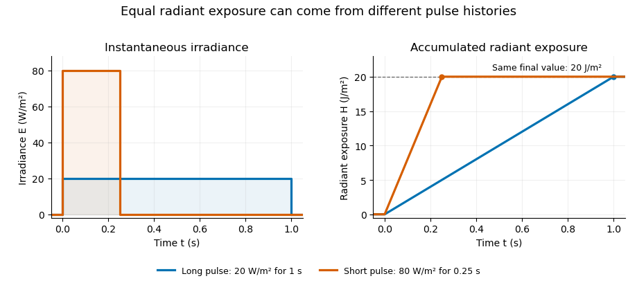
Original rectangular-pulse example: different irradiance histories accumulate the same radiant exposure.
Details. Integrating over a receiving patch gives its incident radiant energy:Here is the spatially averaged radiant exposure, rather than necessarily the local maximum. Uniform illumination is the special case where this spatially averaged radiant exposure equals the local value everywhere on the patch. In the rectangular-pulse example, a uniformly illuminated patch receives .
For an original spatial example, consider a circular Gaussian beam at a fixed transverse plane, with constant Gaussian beam radius throughout the pulse. Let be its total radiant power and its laser pulse energy. Integrating its transverse irradiance in time gives the radiant exposure of a Gaussian beam:The normalization follows by integrating from to . The disk of radius contains only , so its actual spatially averaged radiant exposure is , not . With stipulated and , the peak is , while the average inside that disk is . State the Gaussian beam radius convention and the receiving area with any reported value.
An energy readout alone therefore does not specify a surface's radiant exposure. In an ideal linear model for pulse energy measurement with a photodiode, dark-subtracted photocurrent has constant spectral responsivity at the chosen wavelength. Integrating the electric current gives signal electric charge . If a known patch of area is uniformly illuminated and all of its incident energy is collected, thenAs a separate stipulated example, and correspond to . Uniform illumination over gives . Background subtraction, collection geometry, detector linearity and an integration window covering the full response are part of this measurement model. Continuous-wave responsivity alone does not establish linearity for a short pulse: silicon-photodiode experiments have observed pulse-dependent saturation.[ref]
Measuring Pulse Energy With Solid-State Photodiodes by Robert E. Vest and others. Abstract: pulsed nonlinearity and dependence on reverse bias and illuminated area
A historical NIST measurement calibration separates these operations experimentally. A modulator produces pulses from a continuous-wave laser; a calibrated beam splitter sends one beam to a slow thermal reference and another to the pulse detector. The reference records the accumulated energy, while the pulse repetition rate and injection duration determine the mean energy per pulse. The detector's integrating electronics provide a pulse-energy readout. Converting such a readout to radiant exposure additionally requires the illuminated area and its spatial distribution.[ref]
The beam-use term fluence denotes the same time integral for a directed beam normal to the chosen surface. For light arriving from many directions, specify the angular geometry: planar irradiance and spherical irradiance are different quantities, so a value defined using one cannot simply be substituted for the other.[ref]
International Lighting Vocabulary by CIE. Entry 17-21-054, notes 1–2: directional radiance and the small-sphere construction
Radiant energy is the amount of energy emitted, transferred or received as electromagnetic radiation. It is measured in joules. For the specified beam or collection of rays crossing a boundary,where radiant flux is radiation power. The receiving geometry and time interval are part of the statement; dividing by a receiving area produces radiant exposure, rather than another total energy.[ref]
International Lighting Vocabulary by CIE. Entry17-21-041, definition and notes1 and4
For an original passive-optic example, stipulate incident during an interval, with no remaining change of stored energy afterward. Suppose is transmitted, reflected and absorbed. Their sum is the incoming . A detector collecting only the transmitted path receives , even though the source supplied more. This radiometric energy balance specifies the collection boundary instead of equating every energy readout in the apparatus.
A thermal detector converts absorbed radiation into an observable temperature response; a calibrated model relates that response to received energy. A documented NIST arrangement uses a slow thermal reference and calibrated beam splitting to establish pulse-energy measurements.[ref]
Calibration Service for Low-level Pulsed-Laser Radiometers at 1.06 µm: Pulse Energy and Peak Power by Rodney W. Leonhardt. §3.4, printedp.6; §4, printedpp.9–10
Absorbed energy, incident radiant energy and energy in an uncollected branch must remain distinct in that calibration.Two sources can deliver the same radiant energy with different radiant flux histories or spectra. Their total energies agree only for the specified integration and collection; this alone does not determine peak power, radiant exposure at a point or detector response.
Spherical irradiance counts incident radiance from all directions without selecting a receiving-plane normal. Using the projected-area convention specified in the CIE entry's note2,Here is an element of solid angle. An ideal small sphere of radius intercepts radiant flux . The denominator is its diametrical projected area, not its full surface area.[ref]
International Lighting Vocabulary by CIE. Entry17-21-054, note2, small-sphere construction; note5, units
For an original isotropic radiance field example, take in every direction. Then . A one-sided plane instead receivesThe factor four follows from the different angular geometries; it is not a unit conversion. Averaging the sphere's intercepted power over its actual surface also gives , rather than the projected-area-normalized quantity above.
An all-direction receiver must have a characterized angular response. A single flat irradiance detector inherently samples a hemisphere with projected-area weighting, so rotating it or enclosing it in a diffuser does not supply an all-direction value without an appropriate response model and measurement calibration. Report the angular and area conventions with the result; equal units do not make irradiance and spherical irradiance interchangeable.
An integrating sphere is an optical cavity with diffusely reflecting interior walls and ports for illumination, samples or detectors. Repeated wall reflections mix the incident radiant flux, reducing sensitivity to where it first strikes. Baffles prevent a receiver from directly viewing an unwanted source or illuminated patch; port size and wall reflectance remain part of the response model.[ref]
An original encounter model illustrates the effect of openings. Suppose a well-mixed reflection retains fraction and fraction of the reflected light escapes through ports before the next wall encounter. The integrating-sphere port-loss factor combines with wall reflectance to give a survival fraction . If the first wall encounter carries energy , successive encounters carry , so their summed incident energy is .
With stipulated and , this sum is . Enlarging the openings to reduces it to . These are repeated encounters with the same initially supplied energy, not optical gain: absorption and escape together still account for that original energy. The example counts incident wall encounters from the first one and does not assert a calibrated detector multiplier.
An actual sphere measurement compares its detector signal with a calibrated input or reference. Coating wavelength dependence, ports, sample substitution and temporal response can affect the conversion. The primary guide discusses reflectance/transmittance arrangements and their measurement geometry.[ref] An integrating sphere is therefore useful apparatus, rather than a guarantee that every outgoing component has been measured without correction.
Pinned article: Introduction to the OurBigBook Project
Welcome to the OurBigBook Project! Our goal is to create the perfect publishing platform for STEM subjects, and get university-level students to write the best free STEM tutorials ever.
Everyone is welcome to create an account and play with the site: ourbigbook.com/go/register. We belive that students themselves can write amazing tutorials, but teachers are welcome too. You can write about anything you want, it doesn't have to be STEM or even educational. Silly test content is very welcome and you won't be penalized in any way. Just keep it legal!
Intro to OurBigBook
. Source. We have two killer features:
- topics: topics group articles by different users with the same title, e.g. here is the topic for the "Fundamental Theorem of Calculus" ourbigbook.com/go/topic/fundamental-theorem-of-calculusArticles of different users are sorted by upvote within each article page. This feature is a bit like:
- a Wikipedia where each user can have their own version of each article
- a Q&A website like Stack Overflow, where multiple people can give their views on a given topic, and the best ones are sorted by upvote. Except you don't need to wait for someone to ask first, and any topic goes, no matter how narrow or broad
This feature makes it possible for readers to find better explanations of any topic created by other writers. And it allows writers to create an explanation in a place that readers might actually find it.
Figure 1. Screenshot of the "Derivative" topic page. View it live at: ourbigbook.com/go/topic/derivativeVideo 2. OurBigBook Web topics demo. Source. - local editing: you can store all your personal knowledge base content locally in a plaintext markup format that can be edited locally and published either:This way you can be sure that even if OurBigBook.com were to go down one day (which we have no plans to do as it is quite cheap to host!), your content will still be perfectly readable as a static site.
- to OurBigBook.com to get awesome multi-user features like topics and likes
- as HTML files to a static website, which you can host yourself for free on many external providers like GitHub Pages, and remain in full control

Figure 2. You can publish local OurBigBook lightweight markup files to either OurBigBook.com or as a static website.
Figure 3. Visual Studio Code extension installation.
Figure 5. . You can also edit articles on the Web editor without installing anything locally. Video 3. Edit locally and publish demo. Source. This shows editing OurBigBook Markup and publishing it using the Visual Studio Code extension. 
- Infinitely deep tables of contents:



All our software is open source and hosted at: github.com/ourbigbook/ourbigbook
Further documentation can be found at: docs.ourbigbook.com
Feel free to reach our to us for any help or suggestions: docs.ourbigbook.com/#contact