For a slender winding around a toroid with $N$ turns, core area $A$, mean magnetic path length $\ell$ and approximately constant magnetic permeability $\mu$, Ampère's law gives $H\ell =NI$. The linked magnetic flux is $N\Phi =N\mu HA$, so $L=N\Phi /I=\mu N^{2}A/\ell$. This approximation neglects flux leakage and variation across the core and assumes operation below magnetic saturation. With a nonlinear magnetic core, an incremental inductance instead depends on differential permeability at the operating point.

A modern teaching experiment slows gravity-driven motion enough to resolve it with a photogate. PASCO scientific's Inclined Plane Dynamics Set, ME-6966, Instruction Manual 012-10874A describes “Acceleration Down an Incline” on printed pages 15–16. Its apparatus is a GOcar on a PAStrack with an adjustable incline support, a bracket-mounted photogate, a cart-mounted picket fence, and an interface with recording software. For the interface method, the fence's $1\mathrm{cm}$ pattern is aligned to interrupt the beam. Recording starts before release from rest; the cart is caught at the bottom bumper. The procedure specifies three runs per angle, starting at $14^{\circ }$ and reducing by $2^{\circ }$, with the release position fixed. The readout is velocity against time; its slope estimates acceleration. Mean accelerations are plotted against $\sin \theta$, testing the ideal slope $g$. An added-mass comparison is also requested. These are protocol settings, not observed results.^[ref]

The cart undergoes rolling without slipping at its wheels, whereas the worked block undergoes contact slip. Even ideal wheel moment of inertia changes the cart prediction. For total cart mass $M$, wheel radii $r_i$ and axial moments of inertia $I_i$, rigid wheels with fixed axles and no losses giveTo derive it, combine translational kinetic energy $M{v}^2/2$ with wheel rotational kinetic energy ${\sum }_i{I}_i(v/r_i{)}^2/2$, then equate their rate of change to the release of gravitational potential energy $Mg\sin \theta v$. This is the multiwheel counterpart of rolling acceleration with rotational inertia. Neglecting wheel moment of inertia yields $a\simeq g\sin \theta$; treating a cart as a solid rolling cylinder would give a different correction.

Useful additional controls are repeated releases without a push, checking the fence alignment and spacing, and checking that the recorded velocity trace is straight over the fitted interval. A gently moving cart on a level track can expose losses or unintended tilt. These checks help distinguish an angle or timing error from neglected wheel moment of inertia, bearing friction, or drag force. The three-run spread measures repeatability but cannot by itself reveal a shared calibration error. The inspected protocol makes the gravity component measurable; it does not measure the sliding block's coefficient of kinetic friction.

First test rest. With no other tangential forces, the required uphill static friction is $f_s=mg\sin \theta$. Its maximum is ${\mu }_{s}N$, where ${\mu }_s$ is the coefficient of static friction. ThusThe tangent function is increasing on this angle range, and its inverse tangent determines the last permitted resting angle ${\theta }_c$. At equality, the ideal model still permits limiting rest; a larger angle excludes it. Below the threshold, setting $f_s={\mu }_{s}N$ would incorrectly impose the maximum static friction even when less is required. Static friction on an inclined plane and inclined-plane measurement of static friction develop this onset criterion further.

For a block already sliding downhill, uphill kinetic friction has magnitude $f_k={\mu }_{k}N$, where ${\mu }_k$ is the coefficient of kinetic friction. Taking downhill as positive, Newton's second law becomesEvery term in the force balance scales with mass; division by $m>0$ removes it. Doubling mass doubles both gravitational weight and the contact forces, while leaving this acceleration unchanged if the coefficients remain unchanged. A mass-independent result is a prediction of these assumptions, rather than a universal property of every ramp.

For an original numerical model, stipulate $m=3\mathrm{kg}$, $g=9.8m/{\mathrm{s}}^2$, ${\mu }_s=0.45$ and ${\mu }_k=0.30$. The critical angle is ${\theta }_c\simeq 24.23^{\circ }$. At $20^{\circ }$, the normal force is $27.627\mathrm{N}$; rest requires $10.055\mathrm{N}$ of uphill static friction, below its $12.432\mathrm{N}$ bound. A resting block can stay there. If it is already sliding downhill, however, the kinetic friction is only $8.288\mathrm{N}$, giving downhill acceleration $a\simeq 0.5891m/{\mathrm{s}}^2$. Specifying the initial state matters.

At $30^{\circ }$, the downhill component of gravitational weight is $14.700\mathrm{N}$, while $N\simeq 25.461\mathrm{N}$ and the static friction bound is only $11.458\mathrm{N}$. Rest is impossible. During downhill sliding,Released from rest on a sufficiently long ramp, this ideal block covers its first $1.00\mathrm{m}$ in $t=\sqrt{2L/a}\simeq 0.9218\mathrm{s}$, reaching speed $v=\sqrt{2aL}\simeq 2.1697m/s$. As an independent energy calculation, the lost gravitational potential energy is $mgL\sin \theta =14.700\mathrm{J}$ and kinetic friction removes $f_{k}L\simeq 7.638\mathrm{J}$ of mechanical energy. The remaining $7.062\mathrm{J}$ equals $m{v}^2/2$ by the work-energy theorem.

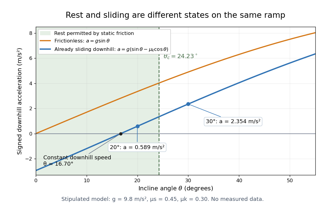
At $\theta =\arctan {\mu }_k$, downhill sliding has zero acceleration and therefore constant velocity. Below that angle, a downhill-moving block slows; when it stops, test the static friction bound again. For uphill sliding, kinetic friction points downhill, so the signed downhill acceleration instead is $g(\sin \theta +{\mu }_k\cos \theta )$. The sign follows contact slip, and the downhill formula cannot be used unchanged after a reversal.

Choose a unit vector ${\mathbf{e}}_d$ pointing downhill and a perpendicular unit vector ${\mathbf{e}}_n$ pointing outward from the inclined plane. The gravitational weight points vertically downward. Its scalar projections onto these directions giveThe angle between the downward vertical and the inward normal is $\theta$: the inward component uses cosine, and the downhill component uses sine. These are two components of one force. They replace its vertical arrow in a component calculation; adding them to that same arrow would count gravitational weight twice.

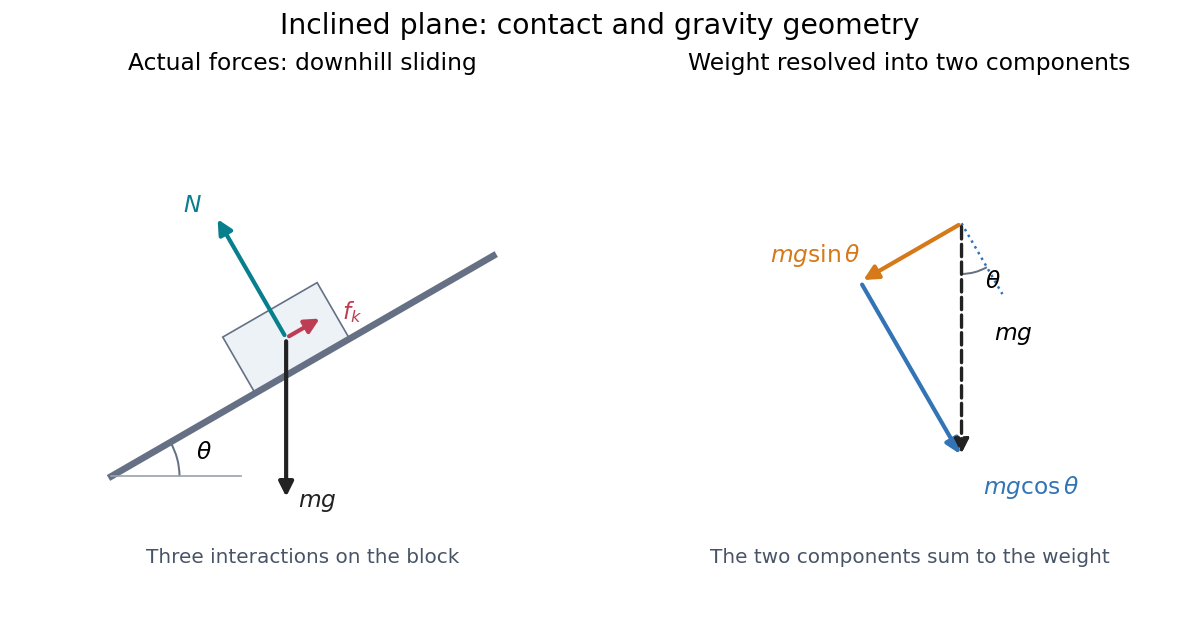
Continued contact with a stationary straight inclined plane gives zero perpendicular acceleration. The perpendicular component of Newton's second law therefore givesThis is why the normal force generally differs from $mg$: it balances the inward component, rather than the whole gravitational weight. An extra lifting force, a curved surface, or motion of the support would require a new perpendicular balance.^[ref]

The same geometry explains the ramp's usefulness. A frictionless block pulled uphill at constant velocity needs a parallel force $P=mg\sin \theta$. Travelling a distance $L$ raises it through height $h=L\sin \theta$, so the pulling work is $PL=mgh$, its gain in gravitational potential energy. The smaller force costs a larger displacement; the work-energy theorem keeps the accounting consistent.

The antibody hinge region is a flexible IgG immunoglobulin heavy chain segment between $C_{H1}$ and $C_{H2}$ containing inter-heavy-chain disulfide bonds.^[ref]

Gerald M. Edelman reduced IgG disulfide bonds and used dissociating chemical solutions, including $6\mathrm{mol}{\mathrm{L}}^{-1}$ urea. Ultracentrifugal analysis showed a decrease in molar mass, supporting a multichain protein. In the comparison reproduced in his lecture, starch gel electrophoresis in urea separated serum IgG and a urinary protein from the same patient, alongside their reduced and alkylation-treated preparations. The untreated samples provided the treatment comparison; the urinary material provided a chain-identity comparison. The treated serum sample revealed heavy- and light-chain bands. Two-dimensional peptide mapping compared the urinary protein with the isolated immunoglobulin light chain. Together these readouts supported a shared chain identity.^[ref]

The controls address distinct alternatives. Treatment-dependent separation supports chains joined in the starting protein; a matching gel electrophoresis position alone would not uniquely identify a chain. Agreement of peptide mapping adds an independent chemical comparison. Neither readout gives atomic coordinates, and this patient's preparation does not establish a common protein primary structure for all antibodies.

Reduction targets protein disulfide bonds, while protein denaturation weakens the folded assembly. Neither operation is the proteolysis that cuts peptide bonds. This explains why chain separation and Papain digestion of IgG give different inventories: four intact chain backbones in the first case, three assembled fragments in the second.

The Mixture measurements and the Gibbs-Duhem constraint article describes the inspected acetone–chloroform preparation, apparatus, paired readouts, controls and sampling limits.^[ref]

That existing apparatus account supplies the experimental controls and limitations. Its refractive index calibration yields mass fractions, which must be converted to mole fractions. For a measured component-A mass fraction $w_A$ and component molar masses $M_A,M_B$,Apply this conversion separately to the flask sample and to completely condensed vapor to obtain $x_A$ and $y_A$. Comparing $y_{i}P$ with $x_i{p}_i^{\ast }(T)$ tests Raoult's law at the measured temperature; using the changing temperature at each composition is essential. The chosen A/B values above are unrelated to the protocol's substances.

The more general diagnostic, retaining an ideal gas vapor and negligible pure-liquid pressure correction, isThis follows by replacing $\ln x_i$ with $\ln (x_i{\gamma }_i)$ in the chemical potential subtraction used for Raoult's law. A reproducible discrepancy from ${\gamma }_i=1$ can expose failure of the ideal solution approximation, but interpreting it requires checking measurement uncertainty, representative paired sampling and the ideal gas approximation. Apparent agreement within uncertainty supports an approximation over the tested conditions; it cannot establish exact ideality at every composition.

Positive or negative deviations of component partial pressures require activity coefficients different from one under these assumptions. An azeotrope is also absent from the chosen unequal-vapor pressure model: the explicit inequality in ideal binary vapor composition gives $y_A>x_A$ throughout $0<x_A<1$. An interior equality would require $p_A^{\ast }=p_B^{\ast }$; in that degenerate case every composition has $y_A=x_A$, rather than an isolated enrichment reversal. Neither an azeotrope nor liquid phase separation should be inferred from the ideal curves.

The Gibbs free energy of mixing compares the final mixture's Gibbs free energy with that of its initially separate components at the same temperature and pressure. For an ideal solution, subtract the pure-component reference from $G={\sum }_i{n}_i{\mu }_i$:For one mole of the chosen A/B ideal solution at $300\mathrm{K}$ and $x_A=0.4$,The individual chemical potential changes are $RT\ln 0.4\approx -2.28554\mathrm{kJ}\mathrm{mo}{\mathrm{l}}^{-1}$ for A and $RT\ln 0.6\approx -1.27417\mathrm{kJ}\mathrm{mo}{\mathrm{l}}^{-1}$ for B. Weighting these by $0.4\mathrm{mol}$ and $0.6\mathrm{mol}$ reproduces the total Gibbs free energy of mixing.

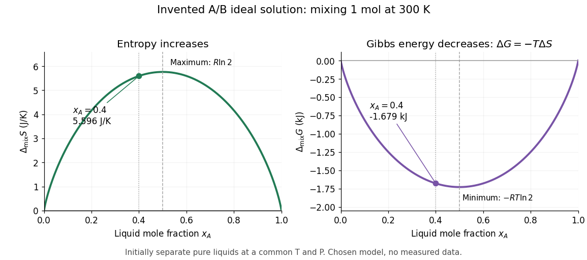
If ideality holds in a neighborhood of the specified temperature and pressure, differentiation at fixed component amounts givesThus the ideal mixing Gibbs free energy decrease comes entirely from the entropy increase; the mixing enthalpy and volume changes vanish. Ideality at a single isolated state alone does not determine temperature or pressure derivatives.^[ref]

The same formula rules out spontaneous separation into two liquid thermodynamic phases within this model. Per mole, the mixing Gibbs free energy $g_{\mathrm{mix}}=RT[x\ln x+(1-x)\ln (1-x)]$ hasAdding the pure-component reference contributions changes only a term linear in $x$. The total molar Gibbs free energy is therefore a strictly convex function: a separated pair of different compositions has a larger composition-weighted Gibbs free energy than the uniform sample with the same inventory. Such phase separation requires physics beyond this ideal solution model.

The entropy of mixing is the entropy change between initially separate components and their final mixture, with initial and final temperatures, pressures and component amount of substance values specified. For an ideal solution made from pure liquids at the same temperature and pressure, let $n={\sum }_i{n}_i$. ThenThe right-hand expression is the ideal solution result; the general definition does not require ideality. Each interior mole fraction has a negative logarithm, so mixing distinct components gives positive entropy of mixing. At a pure endpoint, use the limit $x\ln x\to 0$ as $x\to 0^{+}$.

For one mole of the chosen A/B ideal solution with $x_A=0.4$,For the same total amount of substance, equal mole fractions maximize this binary entropy of mixing: the composition function $s(x)=-x\ln x-(1-x)\ln (1-x)$ hasso its unique maximum is $s(1/2)=\ln 2$. This is a comparison between different prepared compositions, not a prediction that a closed sample changes its component inventory to become equimolar.

In the ideal solution and ideal gas vapor approximation, each component's partial pressure equals its liquid mole fraction times its pure-component vapor pressure at the same temperature:These pressure formulas neglect the change in the pure-liquid reference between its saturation pressure and $P$; appreciable real gas behavior also requires a more general treatment. The ideal solution definition in terms of chemical potentials does not require either approximation.^[ref]

A short derivation explains the reference choice. At vapor-liquid equilibrium, each component has the same chemical potential in the liquid and vapor. For an ideal gas mixture, chemical potential of an ideal gas giveswhere $p^{\circ }$ is a reference pressure. Approximate ${\mu }_i^{\ast }(T,P)$ by ${\mu }_i^{\ast }(T,p_i^{\ast })$ and subtract the pure-component equation from the mixture equation:Taking the exponential function gives Raoult's law. Summing partial pressures and normalizing gives $P$ and $y_i$; this last step uses the ideal gas vapor assumption separately from the liquid model.

The law is named after François-Marie Raoult, who measured vapor pressures and freezing behavior of chemical solutions.^[ref]

Hexane is an alkane with formula ${\mathrm{C}}_6{\mathrm{H}}_{14}$; the unqualified laboratory name often refers to the straight-chain isomer, n-hexane. Other constitutional isomers share the same formula.

Its mostly nonpolar molecular surface explains its use as a solvent for many hydrophobic substances. Commercial mixtures called hexanes need not be a chemically pure single isomer, so the material name and molecular identity should not be treated as interchangeable.