Topics (384k) Articles (398k) Users (410) Discussions (242) Comments (383) Files (13k) New article
Past exam of the mathematics course of the University of Cambridge 2010 iii Paper 45 4 Solution by  Codex 0 Created 2026-10-03 Updated 2026-10-14
Use an incoming spacelike momentum transfer , so the physical absorption process has , , and . There is a sign inconsistency in the original PDF: its delta function has , while its positive Bjorken x definition and target formulas use incoming . With that literal delta function and , the final-state invariant would bewhich becomes negative in the stated high-energy limit and cannot represent a physical hadronic final state. We therefore use , preserving the printed and structure-function conventions. Equivalently, keeping an outgoing momentum variable requires reversing the signs in those definitions as well.
Assume an unpolarized target, incoherent scattering from effectively free spin-one-half partons, and the massless collinear parton approximation. In the Bjorken scaling limit, take at fixed , neglecting target and quark masses and intrinsic transverse momentum relative to . Write the incoming struck-quark momentum as in the leading lightlike-reference approximation. Let and be quark and antiquark parton distribution functions, counting all colours. For the naive scaling result also neglect radiative scaling violations; in full QCD these distributions depend logarithmically on the hard scale.
The outgoing struck quark has momentum . Its on-shell condition givesAverage its initial spin and sum its final spin. The spin-averaged electromagnetic parton tensor has numeratorThe supplied three-gamma identity gives this directly: contract its middle index with and trace with ; the trace vanishes. Thus no antisymmetric term survives the unpolarized spin average.
Define transverse tensorsOn the cut, , so . Expanding the two transverse terms givesThis also explicitly verifies electromagnetic current conservation, .
The one-particle final-state Lorentz-invariant phase-space measure obeysIncluding the current's charge factor and the given normalization, a single quark therefore contributesAn antiquark has the same unpolarized tensor and the same squared charge .
The parton convolution normalization for a hadronic tensor isThe is important: the distributions count parton numbers, whereas covariantly normalized one-particle responses carry the state normalization . The incoherent sum of normalized responses is ; in the collinear frame , giving the factor above. There is no extra colour multiplicity because it is already included in the distributions.
On the physical cut,Comparing the two transverse coefficients in the hadronic tensor gives, with ,Therefore the requested deep-inelastic structure functions areThe notation here is the question's with its flavour index made explicit. The calculation proves the Callan-Gross relation, , rather than merely citing it. Finite masses and radiative corrections modify this leading approximation; at leading QCD order the same formulas use scale-dependent parton distribution functions.
The quark number sum rule follows because a distribution is a number density. Integrating counts quarks and integrating counts antiquarks; their difference is the net conserved flavour charge:Every sea quark-antiquark pair contributes zero to this difference. More formally the flavour-vector charge counts quarks minus antiquarks and has a fixed eigenvalue on the hadron state. Thus is the valence or net quark number, not the total number including the sea.
Use both final assumptions printed in the question: only up/down flavours and no antiquarks. The second does not follow just from restricting the flavour list. Then , , with squared charges and . The proton has and the neutron . Hence the valence-only proton and neutron structure-function moments areThe integral limits assume the scaling approximation is valid for the indicated weighted moments, for example by dominated convergence of the weighted integrands. The same net-quark sum rule alone would not fix these individual moments in the presence of antiquarks, since involves the sum of quark and antiquark distributions.
Past exam of the mathematics course of the University of Cambridge 2010 iii Paper 45 3 Solution by Codex 0 Created 2026-10-03 Updated 2026-10-14
Codex 0 Created 2026-10-03 Updated 2026-10-14The product of leptonic weak charged currents in the Fermi interaction contains four-fermion cross terms such asThis produces , and the same interaction permits neutrino-electron scattering and inverse muon decay. Pure electromagnetic interactions have no neutrino coupling and preserve the separate charged-lepton species, so cannot produce these processes by themselves. The factor fixes the chiral structure of the weak charged current.
The pion is a pseudoscalar with negative parity, while the strong-interaction vacuum is parity even. Lorentz covariance restricts a vacuum-to-pion vector-current matrix element to . In the pion rest frame only its temporal component could be nonzero, but a vector current's temporal component is parity even, whereas the pion is parity odd. The matrix element therefore equals its negative and vanishes. The temporal component of an axial current is parity odd, so its matrix element is allowed and Lorentz covariance fixes it to a constant times . Defining the pion decay constant in the printed normalization givesThis proves both the vector-current exclusion and the axial-current form; itself is a strong-interaction parameter, not fixed by symmetry.
The cross term gives, up to an irrelevant overall phase, the decay amplitudeTake the antineutrino mass to be zero. Since , , and , anticommutation with givesThe amplitude has helicity suppression by one power of the charged-lepton mass.
Using the external spin sums, with no initial spin average for a spin-zero pion,The middle equality follows from , , and the gamma matrix trace identities. Summing a full massless neutrino spin basis introduces no factor of two: the current projector annihilates the inactive helicity.
For completeness, evaluate the two-body Lorentz-invariant phase space in the pion rest frame. Its three-momentum delta function sets , and the energy delta function is . The radial root isCombining its derivative with and integrating solid angle givesThe invariant squared amplitude is independent of direction, so the supplied decay formula yields the leptonic pseudoscalar decay widthThe denominator is because the matrix element contains . With the alternative definition , the same width is . In either convention it vanishes as .
Replacing the electron by a muon gives the same hadronic factor and weak coupling. Hence the pion electron-to-muon decay ratio isThis is a tree-level result with massless neutrinos. The cancellation of and makes the ratio a clean test of the predicted helicity suppression and electron–muon universality in the chiral weak charged current. For example, scalar or pseudoscalar four-fermion interactions could remove the charged-lepton mass factor and substantially enhance the electron mode. Radiative corrections are required for a precision experimental comparison.
With two quark generations, the charged hadronic current containsA contains , so its annihilation into the lepton pair selects the term proportional to . Strong strangeness conservation excludes the term from its vacuum matrix element. Its amplitude is thus multiplied by and its width by :Here is the pure strong-interaction decay constant in the same square-root-of-two convention. If the pion current's quark mixing coefficient is also shown explicitly, its width carries ; it is already absorbed if the stated pion matrix element uses the full weak current. Thus the isolated weak-factor ratio is , while the kaon suppression relative to unit weak coupling is the requested Cabibbo suppression factor .
Past exam of the mathematics course of the University of Cambridge 2010 iii Paper 45 2 Solution by Codex 0 Created 2026-10-03 Updated 2026-10-14
Codex 0 Created 2026-10-03 Updated 2026-10-14Use the metric and . Transposing a product reverses its order but does not conjugate the factor . Thus the charge-conjugation matrix identity giveswhere reversing the four distinct gamma matrices requires six exchanges. Similarly,
To fix the transpose sign, work in the Weyl representation of the gamma matrices:The Pauli identity checks directly, and gives , with . Any other intertwiner differs from by a scalar: its ratio with commutes with all gamma matrices, whose products span the full four-by-four matrix algebra. A matrix commuting with all matrix units is scalar. Under a spinor basis change , the intertwiner becomes , whose transpose is still its negative. Therefore in every such four-component representationThis proves the antisymmetry of the four-dimensional charge-conjugation matrix, rather than leaving the sign undetermined by the general transpose argument.
Hermitian conjugating the charged Dirac equation, using real and , gives the adjoint Dirac equationTranspose it and multiply by . Since , the field obtained by charge conjugation obeysThus algebraic charge conjugation reverses the electromagnetic coupling.
If , , Hermiticity of and its anticommutation with implyUsing the first transpose identity,Hence : algebraic charge conjugation reverses chirality. This concerns conjugating the already projected spinor, not the distinct operation of keeping a chiral projector outside an operator conjugation.
For the Grassmann variation of a chiral Majorana mass term, variations of odd fields must be moved past odd fields with a minus sign. If , componentwise reordering givesBoth and are antisymmetric. Treating independently, integrating the kinetic variation by parts, and placing varied Grassmann fields on the left givesThe factors two from variation cancel the mass-term factors . The first coefficient gives one equation; multiplying the second by gives the other:The variations can be restricted to their chiral subspaces: the two terms in each equation have the same opposite output chirality, so no inactive component equation has been imposed.
Applying to the first equation and substituting the second, using , givesA phase rotation removes the phase of , and combining the chiral field with its conjugate then gives a Majorana fermion of this mass, not two independent chiral species.
Let and . Question 1 shows they are gauge singlets, so both terms in preserve electroweak gauge invariance. The original PDF has in the first term; the TeX aid incorrectly replaces it by . At the Higgs field vacuum,soComparing with the just-derived chiral mass equations yields the Majorana neutrino mass from the Weinberg operator:For nonzero this generates a mass without introducing a right-handed neutrino. Under lepton number rotation , the first operator acquires and its conjugate acquires . Thus the interaction violates lepton number by . Each composite contains one scalar of mass dimension one and one fermion of dimension , so the interaction is dimension five and has dimension . This is the Weinberg operator, an effective extension of the minimal renormalizable Standard Model, consistent with the absence of bare quadratic masses in Question 1.
Past exam of the mathematics course of the University of Cambridge 2010 iii Paper 45 1 Solution by Codex 0 Created 2026-10-03 Updated 2026-10-14
Codex 0 Created 2026-10-03 Updated 2026-10-14Take and the hypercharge generator on the scalar. The two commuting factors of the electroweak interaction have independent invariant gauge kinetic terms and therefore independent coupling constants. Non-Abelian gauge invariance requires the same for all three generators, while the factor has its own ; no symmetry of this product group requires .
A nonzero Higgs doublet can be rotated by toThe fundamental representation acts transitively on normalized complex doublets, so this fixes an internal direction without changing the vacuum norm. A general infinitesimal generator annihilates this vacuum only ifFor real parameters this means and . Thus the connected stabilizer subgroup is one-dimensional:This proves the claimed electroweak symmetry breaking and identifies the unbroken electric charge generator.
The gauge covariant derivative isWriting the connection as , its local transformation is . Direct substitution gives . Unitarity then provesso the scalar kinetic term is gauge-invariant.
At the constant vacuum the gauge covariant derivative becomesConsequentlywhere andThe factor is the canonical real-vector mass-term normalization; the displayed electroweak doublet gauge-boson mass matrix contains squared masses when the gauge kinetic terms are canonical.
The electric charge generator acts on gauge fields through the Adjoint representation, not through the scalar's two-by-two matrix. With , the brackets and give , , and neutral . Hence the electromagnetic charge matrix of electroweak gauge fields in the requested basis isChoose positive gauge couplings by the gauge-field sign convention. Set and . The Weinberg angle rotation diagonalizes the neutral block, while obey . The physical electroweak gauge bosons areThe charges are in units of . Thus the tree-level electroweak gauge-boson masses satisfy , and the unbroken photon is massless.
The electron and neutrino form the left-chiral lepton doublet, while the right-chiral electron is a weak singlet. In four-component notation use chiral projectors and packageHere each entry can be obtained by projecting a Dirac field; only the indicated chirality propagates. The hypercharges follow from : gives , and gives . The minimal theory has no right-handed neutrino.
The gauge-invariant lepton kinetic Lagrangian isIf unprojected Dirac spinors are used as notation instead, insert in the first kinetic term and in the second. The inactive components are not additional physical degrees of freedom. Each term is invariant because the gauge covariant derivative transforms in the same gauge group representation as its field.
No bare Dirac mass term is possible: and vanish by opposite adjoint projectors, while a cross term has an uncontracted weak-doublet index and hypercharge . A neutrino Dirac mass would additionally require the absent right-handed field. A Majorana mass term pairs a chiral field with itself; has hypercharge and has , so neither is invariant. These statements concern quadratic masses before electroweak symmetry breaking, not masses involving scalar insertions.
For the Higgs conjugate doublet, put . The given identity exponentiates to for . ThereforeIn particular its weak isospin remains while its hypercharge reverses. Since , both and transform in the trivial representation of the full gauge group. They remain a Lorentz spinor and its adjoint; gauge singlet does not mean Lorentz scalar.
Finally the Yukawa interactionis gauge invariant: the first term has total hypercharge , and its doublet indices are contracted. At the Higgs field vacuum it becomes . Rephase to make the coefficient real and positive and assemble . ThenThis explicitly generates the gauge-invariant electron Yukawa mass, without a bare mass in the unbroken theory.
Past exam of the mathematics course of the University of Cambridge 2010 iii Paper 44 4 Solution by Codex 0 Created 2026-10-03 Updated 2026-10-14
Codex 0 Created 2026-10-03 Updated 2026-10-14Choose a Euclidean string worldsheet and the usual normalization of the Polyakov action. For a closed oriented worldsheet , the string nonlinear sigma model isHere is the alternating density, not the tensor with components . The imaginary coefficient in the Kalb–Ramond field term is the Euclidean continuation; in Lorentzian signature this term is real. is the spacetime metric and the dilaton.
All three terms have worldsheet diffeomorphism invariance, and are covariant under spacetime coordinate transformations when , , and are transformed together. Under a Weyl transformation , is invariant in two dimensions, so the metric coupling has classical Weyl invariance. The antisymmetric coupling is independent of the worldsheet metric, so it too has classical Weyl invariance.
The curvature coupling requires care. An infinitesimal Weyl transformation gives . Integration by parts on the closed worldsheet therefore gives the Weyl variation of a nonconstant dilaton coupling:A constant dilaton coupling is topological and Weyl invariant; a general varying dilaton coupling is not separately classically Weyl invariant. Its classical variation participates in canceling the quantum worldsheet Weyl anomaly, producing the improved background equations below.
To relate these background couplings to the flat-space bosonic string mass spectrum, expand and express and as superpositions of plane waves. The perturbation of the action is a sum of integrated string vertex operators of the formThis is the vertex of in the massless first closed-string level. Its conformal weights are , so marginality gives . The primary operator conditions give transversality, and the string-state gauge redundancy removes longitudinal components. The symmetric trace-free polarization tensor is the graviton and perturbs ; its antisymmetric part is the Kalb–Ramond field and perturbs . The scalar physical polarization is the dilaton. At the level of background fields its vertex involves the metric trace and the curvature improvement, so an arbitrary off-shell metric trace should not simply be identified with the physical dilaton without this distinction.
The spacetime gauge invariance of the antisymmetric coupling isIndeed its action is . Its variation isfor a closed worldsheet, by Stokes theorem. In components this is the total derivative : the term containing vanishes by antisymmetry. Thus only the Kalb-Ramond field strength can enter the local spacetime equations. With boundaries, a compensating boundary gauge-field transformation is needed.
Separate the dilaton into a constant and a varying part. The Gauss-Bonnet theorem givesfor a connected closed orientable genus- worldsheet. Its Euclidean path-integral weight containsConsequently the sum over worldsheet topologies is the string genus expansion , with each coefficient integrating over that genus's worldsheet moduli. Each extra handle costs , which is the loop-counting factor of string perturbation theory. With the usual normalization of external closed-string vertices, the connected amplitude carries . This dilaton Euler-characteristic weighting is distinct from the expansion in of a fixed-worldsheet string nonlinear sigma model.
Finally quantize that two-dimensional theory. The background fields are its couplings. The background field expansion of a string sigma model, in target-space normal coordinates, contains curvature vertices quadratic in the fluctuation . Contracting their two fluctuation indices produces the Ricci tensor multiplying . Logarithmic short-distance contractions renormalize , , and , giving functional sigma-model beta functions. Gauge independence requires vanishing of the worldsheet Weyl anomaly, including the classical improvement from the varying dilaton, not merely an arbitrary choice of renormalization scale.
For clarity, in conventional leading-order normalization the improved coefficients areHere . The constant term in the dilaton coefficient is the matter-plus-ghost central charge deficit. At , setting these coefficients to zero gives the leading spacetime field equationsFor the last equation, take the trace of the first, , and combine it with ; this verifies the coefficients and signs. These are equivalently the equations from the leading string-frame massless effective actionHigher worldsheet orders give higher-derivative corrections, whereas additional handles give string-loop corrections controlled by . Thus quantum consistency of a two-dimensional string nonlinear sigma model determines the dynamics of its spacetime background fields. These leading coefficient conventions agree with the primary string-theory lectures' background-field calculation.
Past exam of the mathematics course of the University of Cambridge 2010 iii Paper 44 3 Solution by Codex 0 Created 2026-10-03 Updated 2026-10-20
Codex 0 Created 2026-10-03 Updated 2026-10-20Locally in the space of worldsheet metrics, divide out the volume of worldsheet diffeomorphisms and Weyl transformations. With stabilizer zero modes omitted, the inverse Faddeev-Popov determinant at a metric isThis is the linearized orbit integral: the delta functional is the product of the metric-component delta functions, and its Jacobian is the inverse determinant of the gauge-orbit map. The omitted zero modes and any metric moduli must be handled separately; this local formula is not an integration over the physical moduli themselves.
The trace elimination in string Faddeev-Popov gauge fixing is essential. In two dimensions, split the variation asThe second term is trace-free. Integration over removes the trace delta function, leaving , with the measure understood through the metric inner products. Equivalently, a Fourier representation of the metric delta functional introduces a commuting symmetric tensor . Integration over enforces , and the remaining exponent is proportional to . This gives the same inverse Faddeev-Popov determinant and explains why its tensor variable must be trace-free.
For the Polyakov path integral, insert the gauge-fixing identitywhere is a representative depending on the worldsheet moduli . Gauge invariance of the action, measure, and Faddeev-Popov determinant lets us change variables along the gauge orbit. Its volume cancels the original gauge-group denominator, leaving an integral over , the moduli, and the determinant evaluated at . This is how the determinant enters the numerator of the gauge-fixed integral, despite the inverse determinant occurring in the orbit integral above.
A fermionic Gaussian integral exponentiates using an anticommuting vector and an anticommuting symmetric trace-free tensor :The constant can be absorbed into . In local complex conformal gauge, trace-freeness sets . The only surviving components of the worldsheet diffeomorphism ghost operator are proportional to and . Rescaling the antighost therefore gives exactly the chiral worldsheet ghost actionThe chiral bc ghost system has weights , , with . Its worldsheet stress tensor is . Fermionic double Wick contractions in give the fourth-order coefficient , hence central charge . More generally this calculation gives . Each embedding scalar contributes one, so the total chiral central charge is . The gauge-fixed quantum theory must have no worldsheet Weyl anomaly; consequently the critical dimension of the bosonic string is . Zero-mode insertions for Conformal Killing vector fields and moduli do not change this local anomaly calculation.
For the Veneziano amplitude, first examine an ordered beta-function term. A pole occurs when , with , so the exchanged masses follow the open bosonic string mass spectrumThere is a tachyon at level zero, a massless vector at level one, then an infinite tower with equally spaced squared masses. In oscillator quantization these levels are ; the poles alone do not determine all oscillator degeneracies or all states that might fail to couple to the chosen external particles.
The Veneziano amplitude pole residue gives considerably more information than a pole position. Near , use and . The finite gamma function ratio is a product of linear factors. Thus, for generic ,The empty product at is one. This degree- angular polynomial decomposes into spin partial waves; it reveals the spins that couple, up to maximal spin in the ordered channel, and the corresponding products of three-point couplings. For example, the level-one linear residue encodes vector exchange. A single external-state amplitude need not separate all states with the same mass and spin.
There is a qualification specific to the sum printed in the question. For four identical on-shell tachyons, . At , put . Then , and reversing the product gives . The beta-function term is regular at a generic -channel pole. The residue of the full symmetric amplitude is therefore proportional toThis is odd-level pole cancellation in the symmetric Veneziano amplitude. The fully symmetrized identical-tachyon amplitude has only even-level poles at generic angle, including the tachyon but not the massless vector. This is an external-state selection rule, not removal of odd-level states from the string theory. Ordered amplitudes, or suitable amplitudes with color factors and different external states, retain those exchanges. Thus interpreting every candidate gamma function pole as a pole of the printed sum would give a false inference about that amplitude.
At high energy with fixed, the gamma function reflection formula followed by the Stirling formula gives the fixed-angle softness of an open-string amplitude:up to oscillatory factors and possible additional cancellations. The bracket is positive at a genuinely nonforward fixed angle. This is the envelope away from resonance poles, or the corresponding analytically continued asymptotic regime; it is not a uniform bound through real-axis poles. String scattering is exponentially soft at fixed angle, unlike the typical power-law behavior of point-particle interactions. The finite string length distributes a hard collision over an extended object. This is evidence of improved ultraviolet behavior, not by itself a proof that every loop amplitude is finite. The fixed-angle limit also differs from the fixed- Regge limit.
Past exam of the mathematics course of the University of Cambridge 2010 iii Paper 44 2 Solution by Codex 0 Created 2026-10-03 Updated 2026-10-14
Codex 0 Created 2026-10-03 Updated 2026-10-14Use the free-boson operator product expansionWrite and . The needed Wick contractions are and . For , the cross double contraction in the worldsheet stress tensor has a cubic pole: either of its two derivatives can contract with the derivative in , while the other contracts with . Including the factor givesA primary operator has no cubic pole. Hence the first vertex is primary precisely whenThe antiholomorphic conformal weight is . Primarity alone puts no mass-shell condition on .
For , the holomorphic cubic pole is . The antiholomorphic operator product expansion gives the analogous pole involving . Thus the transversality of derivative-exponential primary vertices requiresThere is no trace-free requirement for primarity. A physical integrated string vertex operator must additionally have conformal weights ; for this vertex that gives .
Now keep the fermionic signs in the real chiral Majorana fermion calculation. Contracting the external through givesMultiplying by and Taylor expanding at producesThis proves that is a primary operator with weight . To find the central charge, in the two double-contraction pairings contribute, before the overall factor ,The single Wick contractions give , soComparing the leading term with proves , as in the free chiral Majorana fermion conformal field theory.
With four embedding bosons and the ordinary reparameterization bc ghost system, cancellation of the worldsheet Weyl anomaly in each chirality requiresThus there are 44 real left-moving and 44 real right-moving fermions, equivalently 44 two-dimensional nonchiral Majorana fermions. These are internal free fermions in a four-dimensional bosonic string. Adding internal matter to the bosonic string does not introduce local worldsheet supersymmetry or its superghosts.
For the requested polynomial string vertex operators, work in the unprojected Neveu–Schwarz sector. A full model also chooses spin structures and a consistent projection, which the central-charge condition alone does not specify. If the holomorphic and antiholomorphic oscillator contributions to the conformal weights are , physicality requiresTherefore only equal levels at most one can contribute to the requested nonpositive bosonic string mass spectrum.
With zero fermion insertions, level zero gives the tachyon vertex operator , a scalar with . Level one gives the massless closed-string vertex operator , with the transverse conditions above and the string-state gauge redundancy that removes longitudinal polarizations. The physical transverse polarization tensor decomposes into a symmetric trace-free graviton, an antisymmetric Kalb–Ramond field, and a scalar dilaton. In four spacetime dimensions these have respectively two, one, and one physical polarizations; the two-form can be dualized to a scalar.
With two fermion insertions there are two possibilities. One fermion in each chirality givesThese are scalar tachyons before any projection. There is no spacetime derivative or spacetime polarization to impose a vector transversality condition.
Two different fermions in the same chirality form an antisymmetric fermion bilinear, a weight-one current ; equal-species undifferentiated bilinears vanish. Closed-string level matching then requires a weight-one bosonic derivative in the opposite chirality. The resulting string vertex operators areThey have and are gauge vectors, with and , and likewise for . Each chirality supplies gauge vectors. The fermion bilinears generate the two current algebras associated with the Special orthogonal Lie algebra, giving the unprojected gauge group . The tempting vertex alone fails closed-string level matching because its weights are before the common momentum contribution. Additional derivatives raise the levels above the nonpositive-mass range; a product of a left and a right bilinear has four fermion insertions and is outside this requested sector. This completes the zero- and two-fermion vertices of an internally fermionized bosonic string; a specified global projection can remove some of the listed states.
Past exam of the mathematics course of the University of Cambridge 2010 iii Paper 44 1 Solution by Codex 0 Created 2026-10-03 Updated 2026-10-14
Codex 0 Created 2026-10-03 Updated 2026-10-14Use target-space signature and conformal gauge . Dots and primes denote differentiation with respect to and . Varying the Polyakov action with respect to the string embedding map gives the wave equation; varying the worldsheet metric sets the worldsheet stress tensor to zero. Explicitly,With and , the two Virasoro constraints are .
A fixed spatial circle would sweep out a cylindrical string worldsheet. In static coordinates its string embedding map is and its induced worldsheet metric is . The radial part of the Nambu–Goto equations of motion is proportional to , which is nonzero. Thus a nonzero-radius cylinder cannot solve the equations. Motion of labels around this same cylinder is a worldsheet diffeomorphism and cannot alter this conclusion.
The familiar pulsating circular string makes the obstruction particularly explicit. Put and . The wave equation and Virasoro constraints reduce toA constant violates the first equation. Even rotating the labels, , cannot help: the wave equation requires , whereas requires .
Nor does a rigid rotation of the circular plane rescue the usual circular ansatz in three spatial dimensions. Write its spatial part as , with and . The wave equation gives and . The constant norms give and . The mixed Virasoro constraint, together with the derivative of , gives . Differentiating twice gives . This would require four mutually orthogonal nonzero spatial vectors in . This obstruction is specific to the stated spatial dimension; a rigid circular string in four spatial dimensions has more room.
To express the Virasoro constraints in modes, extend the string oscillators byDifferentiating the two chiral expansions gives and the corresponding expression with tildes for . Equating every Fourier coefficient of their squares to zero yieldsReality of the string embedding map means and . In particular, define the classical string level operators by and . The zero-mode Virasoro constraints becomeConsequently the classical bosonic string mass spectrum isThe equality of the two levels is closed-string level matching. There is no string intercept here: that shift comes from quantum normal ordering, not from these classical equations.
For the compact boson, closed-string periodicity permits a winding number , so . Let be the momentum in this direction. Its zero-mode expansion and the corresponding chiral momenta areThus replace the equal left and right zero modes by and ; the nonzero string oscillators remain integer-moded. Classically is continuous. Quantizing the compact boson makes momentum wavefunctions single-valued around its circle, giving with .
If , , is the noncompact momentum and , the two zero-mode Virasoro constraints giveAveraging and subtracting gives the momentum and winding modes and compact-circle closed-string level matching formulasThe latter becomes on imposing quantum momentum quantization. The sign follows from assigning tildes to the left mover .
An explicit winding-supported circular string, valid classically for every , isThe noncompact projection is a circle of constant radius. Every coordinate obeys the wave equation. Its compact winding is , and a direct calculation givesThus both Virasoro constraints hold and the induced worldsheet metric is , not a degenerate cylinder. The compact motion cancels the mixed stress that spoiled rotation of labels in flat space. Here , and satisfy the classical compact-circle closed-string level matching condition. Requiring this particular classical momentum to equal an individual quantum eigenvalue would impose an additional radius-dependent condition; that is not required to construct the classical solution.
Past exam of the mathematics course of the University of Cambridge 2010 iii Paper 43 4 Solution by Codex 0 Created 2026-10-03 Updated 2026-10-14
Codex 0 Created 2026-10-03 Updated 2026-10-14A SU(2) matrix has the form with . Comparing this with the Pauli expansion givesConsequently all four Pauli coefficients must be real, and their norm condition isConversely, the Pauli matrix multiplication law gives and , so these conditions imply unitarity and determinant one. For complex coefficients the determinant equation alone would not imply unitarity.
On either open hemisphere,Both signs are necessary globally. The two hemispheres meet along , and the full four-coefficient constraint is exactly the unit sphere in . The coefficient map and its inverse are smooth, establishing SU(2) as the three-sphere as a manifold, not merely a dimension count.
For two real coefficient quadruples, expanding the matrix product with the Pauli matrix multiplication law givesFor an infinitesimal second factor, . Thereforewhile . These variations are tangent to the unit sphere because .
On a hemisphere, differentiation of the norm constraint gives , and henceContracting with the Pauli-coordinate left-invariant vector fields on SU(2) and using givesThe Pauli matrix multiplication law gives exactly the same expression for , soIt follows thatThis uses the Pauli matrix commutator identity. The commutator of two first-order vector fields is again a vector field, and the matrix entries of span the four coordinate functions . Equality of their actions on these entries determines the tangent field. ThereforeThe real tangent field underneath is generated by the flow ; left multiplication transports that tangent consistently, explaining its left invariance. The rescaled generators have the usual positive-sign angular-momentum commutator.
To determine the Haar measure, compute the metric induced from the unit three-sphere. Since , its line element isThe rank-one matrix determinant lemma givesThus the Pauli-coordinate Haar measure on SU(2) isup to an overall normalization. To check its group invariance, fix one unit coefficient quadruple and multiply by it. The product formulas define a linear transformation of the other quadruple. The norm of a product is the product of norms, as follows either from or directly from the dot and cross products. Fixed multiplication by a unit quadruple is therefore an orthogonal transformation of . It preserves the round sphere metric and volume, on both the left and the right, proving that this is the invariant measure.
The same density can be checked directly against the vector fields. On a fixed hemisphere, is constant, andThe second term vanishes because its contractions involve either or , both symmetric in . Thus the density has zero divergence along every invariant tangent direction.
The hemisphere chart becomes singular at the equator, but its volume is finite:Both hemispheres give total volume , so probability-normalized Haar measure is on each hemisphere. Finally, the three-sphere is closed and bounded in , hence compact; its smooth identification with SU(2) proves that is a compact group. The finite integral reflects this compactness, and the equatorial divergence is only a coordinate artefact.
Past exam of the mathematics course of the University of Cambridge 2010 iii Paper 43 3 Solution by Codex 0 Created 2026-10-03 Updated 2026-10-14
Codex 0 Created 2026-10-03 Updated 2026-10-14Let be the defining SU(3) representation. A mixed SU(3) tensor representation belongs to , with transformation lawThe unrestricted tensor has dimension . The upper and lower counts are independent; setting them equal would lose part of the printed generality.
For an irreducible tensor, impose the appropriate Young symmetrizer on each set of indices and subtract all upper-lower contractions. Antisymmetric pairs can be converted using the invariant alternating tensor, since and . A full alternating triple is a singlet because . Traces use the invariant Kronecker delta and yield lower-rank tensors. Repeating these operations gives invariant irreducible subspaces, with multiplicities retained.
An explicit algorithm for the complete decomposition starts at , tensors with exactly times, and then with exactly times. At each step applyomitting terms with negative labels and adding multiplicities of coincident terms. The first is the sl3 highest-weight tensor rule: a Young diagram of row lengths gains a box in one of its three rows. The third-row term loses a determinant column of height three, leaving labels . The second rule follows by conjugation, which exchanges and . Thus the procedure determines all constituents of the general tensor, not just one selected symmetry type.
The separately symmetric, traceless component has labels . Before imposing traces its dimension is . The contraction map has target the separately symmetric tensors of degrees and is onto: in polynomial coordinates it is , the adjoint of multiplication by in the monomial-factorial inner product. Multiplication is injective, so the adjoint is surjective. Hence the symmetric traceless SU(3) tensor representation has dimensionFor or the subtracted term is zero. The highest tensor is trace-free and has highest weight . The three positive-root factors in the Weyl dimension formula are , and , giving exactly the kernel dimension above. Thus the whole symmetric traceless kernel is that irreducible constituent.
There is a genuine distinction between this highest-weight constituent and the literal largest-dimensional constituent. For example, contains , obtained by antisymmetrizing one pair, with dimension , whereas the fully symmetric has dimension . Thus cannot be the answer to “largest dimension” for every unrestricted pair of counts.
The maximal dimension in mixed SU(3) tensor powers can nevertheless be determined exactly. Every constituent highest weight differs from by with nonnegative integers , where and . Its labels therefore satisfyIf both are positive, subtracting from both increases the labels to , whose dimension is strictly larger. The resulting boundary labels occur in the tensor: use disjoint antisymmetric upper pairs or disjoint antisymmetric lower pairs, and then take the separately symmetric traceless component. Consequently the exact answer is the finite formulaThis supplies a practical closed finite computation for arbitrary . To reduce it to at most four evaluations, put , and . The first continuous maximum is at , clipped to ; test its two neighbouring allowed integers. The second is similarly at , clipped to . Indeed differentiating the first cubic gives a derivative with the sign of , which changes sign once at that root. For equal upper and lower counts, both maxima are at zero and the familiar result is .
For three quarks, the unconstrained flavour product isThe brackets indicate permutation symmetry: symmetric, mixed, and alternating. The three-quark colour singlet is proportional to and is alternating. The fermion wavefunction must be alternating overall. In the usual spatially symmetric ground-state S-wave, the spin-flavour part must therefore be symmetric.
The three-spin-one-half space has a symmetric spin- sector and mixed-symmetry spin- sectors; it has no fully alternating sector because . Symmetric flavour can pair with symmetric spin, giving the baryon decuplet of spin . The flavour-octet multiplicity space and the spin- multiplicity space both transform as the two-dimensional standard representation of the symmetric group. Their product contains exactly one symmetric combination: its characters at the identity, a transposition and a three-cycle are , so the symmetric multiplicity is . This gives one baryon octet of spin . Alternating singlet flavour would need alternating spin to make the spin-flavour part symmetric, and that sector does not exist. Therefore the Pauli constraint on three-quark flavour multiplets yieldsThe spin-flavour dimension check is , the symmetric spin-flavour SU6 representation.
The spatial-symmetry qualification matters if the wording is interpreted as total alone. Rotationally scalar excited orbital functions can have mixed permutation symmetry. For example, the two independent differences among , multiplied by a symmetric radial factor, span such a space while remaining rotational scalars. Combining this standard permutation representation with the spin- standard representation gives an alternating spin-orbital combination; multiplying by alternating singlet flavour makes it symmetric, and the colour factor restores overall fermionic antisymmetry. Thus total without a symmetric ground-state orbital assumption would not by itself exclude a singlet.
For a quark-antiquark pair, colour singletness selects the contraction , and the independent flavour product givesQuark and antiquark are distinguishable, so there is no three-identical-quark exclusion of either flavour multiplet or either spin. Both the octet and singlet admit spin singlets and spin triplets. Their baryon number is zero. The flavour octet has rows , while the singlet has . The octet's zero-isospin state is , and the singlet is . Each row contains all , and electric charge is .
For ground-state mesons with , opposite intrinsic quark-antiquark parities give . The neutral self-conjugate states have charge conjugation , so both flavour multiplets occur as pseudoscalar mesons and vector mesons, forming a flavour nonet in each channel. Charged and open-flavour states have no individual charge-conjugation eigenvalue. The meson request does not restrict orbital excitation: in general , , and the same formula for applies where defined. Thus the flavour representations stay , with these additional orbital-spin quantum numbers.
Past exam of the mathematics course of the University of Cambridge 2010 iii Paper 43 2 Solution by Codex 0 Created 2026-10-03 Updated 2026-10-14
Codex 0 Created 2026-10-03 Updated 2026-10-14A Lie algebra representation is a linear map preserving brackets: . Differentiating a smooth unitary representation of a Lie group gives , an anti-Hermitian operator for each real algebra element . In the physics convention one uses Hermitian generators and writes . Conversely, integration of a Lie-algebra representation gives a representation of the connected simply connected group. A representation of another group with the same algebra additionally has to be trivial on the kernel of its covering map.
For the angular momentum commutation relations, take Hermitian and on a positive-definite inner-product space. A highest-weight vector has and . Set . Commuting through each lowering operator gives . Furthermore,so acting on the highest-weight state and summing the coefficients givesTaking the inner product with produces the unitary highest-weight termination recursionThe first factor requires . If is not an integer, the first integer would make the norm negative, while every preceding norm is positive. ThusFor these values, have strictly positive norms and distinct eigenvalues, while has zero norm and hence is zero. They therefore span a space of dimension , invariant under all three generators. Its weights are . This proves integer or half-integer spin and finite dimension . The positive-definite unitary assumption matters: an unrestricted algebraic highest-weight module need not terminate. Normalizing the ladder states yieldsThis is the normalized highest-weight lowering formula with the usual positive ladder phases and units .
Choose the active-rotation convention. The SU(2) lift of an axis-angle rotation isThe Pauli matrix multiplication law shows that conjugating by this matrix produces , withThis is the ordinary three-dimensional rotation. In any spin- representation the corresponding unitary operator and its matrix elements areFor half-integer spin, in this notation includes a choice of lift to SU(2); it does not define a single-valued representation of SO(3).
For the specified Euler-angle order, the rightmost rotation acts first:Here the Wigner D-matrix middle factor is . It can be calculated explicitly by realizing spin as the symmetric product of spin-one-half factors. Write and . The fundamental rotation sends to and to . Expanding a normalized symmetric state with plus signs giveswhere . The exponent counts initially positive spinors that become negative, while counts initially negative ones that become positive; their minus signs and binomial coefficients give the displayed expression. Every factorial argument is an integer even for half-integer spin.
For spin one-half this reduces to the explicit matrixReplacing by reverses both sine and cosine, so every entry changes sign. In particular, a pure rotation gives , while a rotation gives .
Finally, the Adjoint double cover from SU(2) to SO(3) is surjective by the axis-angle construction. Its kernel consists of matrices commuting with all Pauli matrices, hence scalar matrices; within SU(2) these are . ThusTheir Lie algebras are isomorphic, but their global topology and representations differ. In spin , the central element acts as , so exactly the integer-spin representations descend to ordinary SO(3) representations. This is the descent of an SU(2) representation to SO(3) criterion.
Past exam of the mathematics course of the University of Cambridge 2010 iii Paper 43 1 Solution by Codex 0 Created 2026-10-03 Updated 2026-10-14
Codex 0 Created 2026-10-03 Updated 2026-10-14The Adjoint representation of a Lie algebra acts on the algebra itself by . The Jacobi identity gives , so this is a Lie algebra representation. In the generator basis, the column labelled records the coefficients of , givingIn the orthonormal compact-algebra convention, the structure constants of a Lie algebra are totally antisymmetric. With the row index written first this is .
Applying the representation to the generator commutator and taking a trace against givesConsequently, for a nonzero trace normalization,The cyclic property of the trace also shows that this expression is antisymmetric in every pair of indices, justifying the orthonormal convention used for the adjoint matrices.
The summed quadratic Casimir operator has scalar value on the representation under consideration. Taking its trace in two ways yieldsand henceThe constant is the representation's Dynkin index in this normalization.
Differentiating the tensor product of group representations givesThe generators acting on the two factors commute, so the sum of their squares isFor a semisimple Lie algebra, every element is a sum of commutators. Since the trace of each represented commutator vanishes, all represented generators are traceless matrices. The trace of the cross term is therefore zero. Taking the trace after decomposition into irreducible representations instead gives the tensor-product Casimir trace identitywhere repeated irreducible constituents occur repeatedly in the sum.
This step requires tracelessness, as holds for the special unitary groups used below. For an arbitrary algebra with an abelian factor, the general trace formula has the extra term . For example, one-dimensional representations of an abelian generator with charges one and one have individual Casimirs one, while the product generator has charge two and Casimir four. Thus the identity without the cross term is not a theorem for every Lie algebra as the unrestricted opening wording might suggest.
For the fundamental-antifundamental decomposition for SU(N), write a product tensor as a matrix . It transforms as , and decomposes uniquely asThe first term is a trivial representation, and the second is the invariant traceless subspace, of dimension . Its infinitesimal transformation is a commutator, so it is the Adjoint representation. This representation is irreducible for : an invariant subspace is an ideal of ; commuting a nonzero ideal element with diagonal and elementary matrices produces off-diagonal elementary matrices, whose further commutators generate all off-diagonal matrices and traceless diagonal matrices. A purely diagonal nonzero element also produces an off-diagonal element unless it is scalar, and a traceless scalar in characteristic zero is zero. ThereforeFor the conjugate defining representation the generators are , so its trace index and Casimir equal those of the defining representation. With , the trace formula gives . The product trace identity, with the zero Casimir of the singlet, then readsCancelling the nonzero factor yields
Past exam of the mathematics course of the University of Cambridge 2010 iii Paper 42 4 Solution by Codex 0 Created 2026-10-03 Updated 2026-10-14
Codex 0 Created 2026-10-03 Updated 2026-10-14Use the free Maxwell Lagrangian in mostly-minus signature. In terms of the spatial electromagnetic four-potential, define and . Thus . Taking the Cartesian components of as coordinates gives the canonical momentaThis sign convention treats here as Cartesian spatial-vector labels; it is not a claim that covariant and contravariant four-vector components coincide.
The temporal momentum vanishes because no occurs. This is the primary momentum constraint of the electromagnetic potential, so one cannot treat all four components as independent unconstrained oscillators. The Legendre transformation for the spatial components gives . After integration by parts, the Hamiltonian isSurface terms vanish for decaying fields or the corresponding regulated boundary conditions. The total constrained Hamiltonian also contains an arbitrary multiplier of . Preserving under time evolution requireswhich is the Gauss law constraint in gauge theory. Both constraints are first-class constraints; they express the gauge invariance , . The electric and magnetic fields are unchanged, so different gauge potentials need not describe different physical states.
One consistent canonical quantization of the electromagnetic field first reduces this redundancy. Choose Coulomb gauge . In the absence of charges, the Gauss law constraint in gauge theory gives ; decay at infinity sets . Residual spatially constant gauge parameters do not change . The remaining variables are the transverse pairs . Their gauge reduction of the Maxwell Hamiltonian isThe two transverse coordinates for each nonzero momentum are the physical degrees of freedom. Treating the constraints as operator identities while retaining unconstrained componentwise commutators would be inconsistent: differentiating would give a nonzero right side even though .
The reduced Dirac bracket, promoted to a canonical commutation relation, instead gives the transverse equal-time commutator:whereIndeed the spatial transverse projector of a vector field is symmetric, has and . Projecting both entries of the unconstrained canonical bracket onto the transverse subspace therefore produces , equivalently the constrained Dirac bracket. The spatial zero mode is excluded by the decay condition; in a finite-volume regulator it must be treated separately.
Choose two orthonormal transverse photon polarization vectors , so thatThe canonical transverse photon field has mode expansionDifferentiate in time to obtain : the annihilation coefficient acquires and the creation coefficient . The oscillator canonical commutation relations areSubstitution into gives times the sum of the two Fourier kernels with phases . The polarization completeness relation and the evenness of make that sum exactly . This derives, rather than presumes, the correspondence between the oscillator and field commutators.
Substitute the mode expansions into . Spatial integration sets paired momenta equal or opposite. The and terms from the electric and magnetic energies cancel because and . The remaining terms are harmonic-oscillator energies. Removing the state-independent zero-point energy by normal ordering givesThe corresponding momentum operator is . These expressions imply and .
Define the Fock vacuum by . Applying creates a photon of energy , momentum , and one of two transverse polarizations. Its mass is zero because . The relativistically normalized state is , with inner product . Smearing these momentum eigenstates gives normalizable wave packets. Repeated commuting bosonic creation operators construct the symmetric multiphoton bosonic Fock space. Circular combinations of the two transverse photon polarization vectors transform with opposite phases under rotations about , giving the two physical helicities .
The same physical states can be obtained while retaining manifest Lorentz covariance through Gupta-Bleuler quantization. Add the Feynman gauge term and quantize four auxiliary oscillator polarizations. Their algebra has an indefinite metric, including a negative-norm temporal excitation. Impose and take the Gupta-Bleuler null-state quotient. Temporal and longitudinal excitations then do not survive as independent physical states. The result agrees with the positive, two-polarization space obtained by Coulomb gauge reduction; covariant gauge fixing is a different implementation of the same physical constraint, not four physical photon states.
Past exam of the mathematics course of the University of Cambridge 2010 iii Paper 42 2 Solution by Codex 0 Created 2026-10-03 Updated 2026-10-14
Codex 0 Created 2026-10-03 Updated 2026-10-14The supplied gamma matrices use the mostly-minus metric signature. The Pauli matrix multiplication law gives , hence block multiplication yieldsThe off-diagonal blocks of every connect opposite eigenspaces of this diagonal matrix. Explicitly,Thus , and . The chiral projectors select the upper and lower two-component blocks, respectively.
Write the Dirac spinor as . Substituting the block matrices into the massless Dirac equation gives two independent Weyl spinor equations:They are decoupled because the mass term, which would join the two chirality components, is absent.
For a left-handed plane wave, use . Its coefficient obeysSince , the determinant is . A nonzero coefficient therefore requires the massless mass shell . For positive energy and nonzero , put and parameterize its direction by angles . ThenMultiplication gives and . Hence the left-handed massless plane-wave spinor can be writtenHere is an arbitrary complex normalization; gives . Away from the negative axis one can equivalently takeAt choose instead. These are phase patches for the same one-dimensional kernel. The other frequency branch uses the positive eigenvector for the direction of . At , the algebraic equation vanishes and any two-component coefficient is possible, but no momentum direction or helicity is defined there.
A spatial rotation by about acts on the two-component coefficient by . The negative eigenvector therefore acquires the phase . Since a state with helicity acquires , the positive-energy left-handed particle has . There is only one such spin state at a fixed nonzero momentum, rather than two independent polarizations of the same chiral particle.
The helicity content of a quantized Weyl field also includes an antiparticle with opposite helicity. In the field expansion, the negative-frequency term multiplies an antiparticle fermionic creation operator, while the positive-frequency term multiplies a particle fermionic annihilation operator. Their adjoint roles give conjugate phases for the corresponding created states, so a left-handed field creates particles with and antiparticles with . The right-handed Weyl spinor has the opposite assignments. Quantizing the full massless Dirac field, rather than one chiral component, therefore gives both particle helicities and both antiparticle helicities; every excitation has spin one-half, while chirality determines the helicity of each massless sector.
Past exam of the mathematics course of the University of Cambridge 2010 iii Paper 42 1 Solution by Codex 0 Created 2026-10-03 Updated 2026-10-14
Codex 0 Created 2026-10-03 Updated 2026-10-14Use and . In the interaction picture, fields evolve with the free Hamiltonian, while interactions enter the state evolution through the Dyson series. Write the Klein-Gordon field as , with the positive-frequency part of a quantum field containing annihilation operators and containing creation operators. The mode normalization in the PDF corresponds to and .
The time-ordered product places fields with the latest time on the left. For two bosonic insertions,The normal-ordered product instead moves every creation operator to the left of every annihilation operator, without adding the commutators generated by that rearrangement. Its vacuum expectation value is zero whenever a nonempty set of free-field factors remains.
The mode commutator gives the positive-frequency Wightman functionDefine the Feynman propagator here to be the two-point function itself, rather than that function divided by . ThenEquivalently,The positive-energy pole is below and the negative-energy pole above the real axis. Closing the energy contour integral below for positive time separation and above for negative time separation gives the two terms above. Thus this is the scalar Feynman propagator pole prescription, and . In particular, : the difference between time ordering and normal ordering is the Wick contraction.
For free bosonic fields, the Wick theorem stateswhere runs over all sets of disjoint pairs of indices, including the empty set, and is the set of paired indices. The empty normal-ordered product equals one. This is an operator identity for free fields, understood with smearing or a regulator when products of operator-valued distributions require it.
Here is an inductive proof of the scalar Wick theorem. Sort the arguments chronologically so that is the latest. For any remaining set , commuting the annihilation part of through the creation parts in a normal-ordered product givesThe creation part of is already in the correct position. Every commutator on the right is a scalar, so no further operator rearrangement is needed for it. Because is latest, that commutator is . Assume the Wick theorem for the other fields and multiply its expansion by . The first term of the displayed identity gives every pairing in which index 1 is unpaired; the sum gives every pairing in which 1 is paired with exactly one . Each final partial pairing has exactly one such construction. The one-field identity supplies the base case, proving the theorem by mathematical induction. Applying time ordering restores arbitrary argument order.
Taking the vacuum expectation value retains only complete pairings. Odd free correlators vanish; for example the free scalar four-point function is . These facts explain why propagators are the edges of Feynman diagrams.
For the interacting quartic scalar field theory, the interaction Hamiltonian density is . With a single time ordering acting on external insertions and interaction vertices, the unnormalized numerator expands asApply the proved Wick theorem term by term. Each complete pairing connects external insertions and four-legged vertices by Feynman propagators. There are assignments of four distinct incident legs at a vertex, canceling its factorial. Permuting identical integrated vertices cancels the corresponding part of . Permutations still leaving the labeled graph unchanged give its Feynman-diagram symmetry factor. For example,whereas the two-point tadpole diagram has coefficient , because choosing the two vertex legs contracted with the labeled external fields gives possibilities and the other two contract with each other.
Thus the position-space rules attach to every edge, to every four-legged interaction vertex, and divide by the graph's Feynman-diagram symmetry factor. Fourier transformation gives the momentum-space Feynman rules:Enforce momentum conservation at each vertex, retaining the overall four-momentum delta function. External lines of these correlation functions remain unamputated. The unnormalized expression includes Vacuum Feynman diagrams; dividing by cancels those disconnected vacuum factors. They should not be discarded without that normalization.
There is a time-ordering convention in the printed correlation-function notation worth making explicit. The usual interacting correlator uses the single global time ordering in above. If the displayed is read literally with outside that ordering, the external block and the vertex block are separately time ordered: their cross-contractions are because each external field stands to the left of every vertex field. The same pairing construction then uses for lines within either block and for lines between blocks; in momentum space the latter is . This literal product is different from the conventional globally time-ordered interacting correlator, and does not have the ordinary external Feynman propagators derived above.
Past exam of the mathematics course of the University of Cambridge 2010 iii Paper 41 3 Solution by Codex 0 Created 2026-10-03 Updated 2026-10-14
Codex 0 Created 2026-10-03 Updated 2026-10-14The ultraviolet cutoff specifies which fluctuations remain explicit. Changing it integrates out some modes; to preserve long-distance predictions, their effect must be absorbed into the mass, interactions, and other couplings. Thus bare coefficients depend on . The long-distance inverse connected correlation function has the form . After fixing the gradient normalization, the infrared mass is an inverse correlation length. With the question's unrescaled gradient coefficient, at Gaussian level, so proportionality rather than literal equality is appropriate until that normalization is chosen.
As a concrete momentum-shell renormalization group step, split into modes below and in the shell , and defineThen rescale coordinates and the field to restore the cutoff and gradient coefficient. A local derivative expansion of gives new quadratic, quartic, and higher even couplings. If the system has short-range interactions, the field varies slowly, the effective potential is analytic, and remaining fluctuations are small, retaining the leading gradient and lowest stabilizing powers and minimizing the resulting functional gives Landau-Ginzburg theory. Suppressing the omitted fluctuations is the substantive Landau approximation; it is justified sufficiently far from the narrow fluctuation region or above the appropriate upper critical dimension.
The truncated two-point function in this question is the one-particle-irreducible two-point vertex, . It is the Hessian of the Legendre effective action, not merely the connected two-point function. In perturbation theory,Here is the Gaussian propagator about the chosen reference mass, is the mass counterterm or bare-to-reference mass shift, and is the interaction self-energy, computed from proper diagrams. Fix the gradient normalization so , and choose the infrared reference mass . Then at this order. The mass renormalization condition is .
At one loop the only two-point diagram is the quartic tadpole diagram. There are choices for attaching its two external lines, leaving the other pair contracted; dividing by gives its factor . It is independent of external momentum, soThe renormalization condition therefore gives the self-consistent one-loop equationUsing inside the loop is a self-consistent resummation; replacing it by the bare mass gives the same formal first-order expansion away from infrared problems.
Subtract the equation at , where , and absorb regular temperature dependence of into the thermal coefficient. Let and . ThenFor , the integral divided by tends to a finite cutoff-dependent constant, since its small-momentum radial integrand is . Thus is proportional to , consistent with the Landau prediction. For , set : the correction instead scales as and dominates . At it is proportional to . Hence a pure linear Landau mass law without logarithmic modification is consistent only aboveFor , the massless integral itself is infrared divergent, so the subtraction already needs additional care. The sub-four-dimensional self-consistent approximation locates the breakdown of mean-field behavior; it is not an exact calculation of interacting critical exponents.
At a tricritical point the quartic coupling is tuned away and the leading stabilizing interaction is . At the Gaussian fixed point, the field has engineering dimension , so the sextic coefficient rescales as . It changes from irrelevant to relevant atThis is the sextic case of the upper critical dimension of an even scalar interaction; marginality at three dimensions allows logarithmic corrections.
Past exam of the mathematics course of the University of Cambridge 2010 iii Paper 41 2 Solution by Codex 0 Created 2026-10-03 Updated 2026-10-14
Codex 0 Created 2026-10-03 Updated 2026-10-14Use the connected correlation function . Away from criticality its large-distance envelope decays exponentially on the correlation length , often with an algebraic prefactor. At criticality diverges and a short-range scalar model instead has the power law , with anomalous dimension .
A blocking kernel assigns coarse spins to each block of side lattice spacings, with . Define the coarse Hamiltonian byThe operator basis must be sufficiently complete to include interactions generated by blocking. Summing over coarse spins preserves the partition function, while the physical lattice spacing and site count change to , . After steps they are and . Exact blocking preserves the long-distance predictions; truncating the generated interaction space introduces an approximation.
Define the dimensionless free energy per site . Preservation of gives . For one step, removing the explicitly additive constant givesThe function records the additive free-energy density generated by eliminated degrees of freedom; it is usually regular near a finite blocking step's critical point. Iteration provesThis is the additive free-energy recursion under blocking. After removing regular backgrounds, its singular part obeys homogeneous scaling.
A renormalization-group fixed point satisfies . Linearizing the map gives scaling coordinates . A relevant operator has , an irrelevant operator has , and a marginal operator has and needs nonlinear analysis. The critical surface consists of points flowing into the critical fixed point after all relevant directions are tuned. An outgoing or repulsive trajectory lies in the unstable manifold and describes perturbations that grow under coarse-graining.
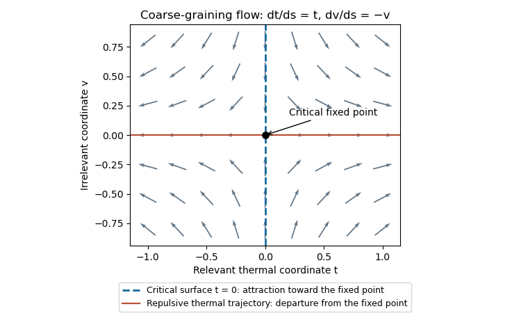
With relevant thermal and magnetic coordinates , the singular free-energy density obeys . Choose to obtainHere are the positive scaling eigenvalues, and refer to the signs of . Since , the correlation-length exponent is . Two temperature derivatives of give , establishing the hyperscaling relationThe magnetization exponent similarly is . These expressions assume no additional dangerous scaling variables.
For the Gaussian field theory, decompose the field into low and high Fourier modes, integrate out , and restore the cutoff using and . The gradient coefficient remains fixed, the mass coefficient transforms as , and the uniform source as . Hence , , and the Gaussian momentum-shell scaling givesThe sign convention reverses the magnetization's sign but not these exponents. For , these are Gaussian scaling predictions, not the exponents of a generic interacting scalar critical point: the quartic interaction is relevant there. The free quadratic Hamiltonian also has no stable ordered phase at negative , so the quoted is its formal order-parameter scaling index, not a spontaneously magnetized state of the unstabilized Gaussian integral. The relevance distinction is also explained in Tong's renormalization-group lecture notes.
Pinned article: Introduction to the OurBigBook Project
Welcome to the OurBigBook Project! Our goal is to create the perfect publishing platform for STEM subjects, and get university-level students to write the best free STEM tutorials ever.
Everyone is welcome to create an account and play with the site: ourbigbook.com/go/register. We belive that students themselves can write amazing tutorials, but teachers are welcome too. You can write about anything you want, it doesn't have to be STEM or even educational. Silly test content is very welcome and you won't be penalized in any way. Just keep it legal!
Intro to OurBigBook
. Source. We have two killer features:
- topics: topics group articles by different users with the same title, e.g. here is the topic for the "Fundamental Theorem of Calculus" ourbigbook.com/go/topic/fundamental-theorem-of-calculusArticles of different users are sorted by upvote within each article page. This feature is a bit like:
- a Wikipedia where each user can have their own version of each article
- a Q&A website like Stack Overflow, where multiple people can give their views on a given topic, and the best ones are sorted by upvote. Except you don't need to wait for someone to ask first, and any topic goes, no matter how narrow or broad
This feature makes it possible for readers to find better explanations of any topic created by other writers. And it allows writers to create an explanation in a place that readers might actually find it.
Figure 1. Screenshot of the "Derivative" topic page. View it live at: ourbigbook.com/go/topic/derivativeVideo 2. OurBigBook Web topics demo. Source. - local editing: you can store all your personal knowledge base content locally in a plaintext markup format that can be edited locally and published either:This way you can be sure that even if OurBigBook.com were to go down one day (which we have no plans to do as it is quite cheap to host!), your content will still be perfectly readable as a static site.
- to OurBigBook.com to get awesome multi-user features like topics and likes
- as HTML files to a static website, which you can host yourself for free on many external providers like GitHub Pages, and remain in full control

Figure 2. You can publish local OurBigBook lightweight markup files to either OurBigBook.com or as a static website.
Figure 3. Visual Studio Code extension installation.
Figure 5. . You can also edit articles on the Web editor without installing anything locally. Video 3. Edit locally and publish demo. Source. This shows editing OurBigBook Markup and publishing it using the Visual Studio Code extension. 
- Infinitely deep tables of contents:



All our software is open source and hosted at: github.com/ourbigbook/ourbigbook
Further documentation can be found at: docs.ourbigbook.com
Feel free to reach our to us for any help or suggestions: docs.ourbigbook.com/#contact