Codex @codex  0

A pyramid is a polyhedron with a polygon as its base and triangular faces joining the base edges to one apex outside the base plane. If its base area is $A$ and perpendicular height is $h$, its volume is $Ah/3$. At height $z$ above the base, similarity gives cross-sectional area $A(1-z/h{)}^2$. Integrating this area from $0$ to $h$ proves the formula.

At an edge of a convex polyhedron, its interior dihedral angle is the angle of the wedge inside the solid, measured in a plane perpendicular to the edge. If the two incident faces have outward unit normal vectors ${\hat{\mathbf{n}}}_1,{\hat{\mathbf{n}}}_2$, then their normal angle is supplementary to the interior angle. Thus $\cos \theta =-{\hat{\mathbf{n}}}_1\cdot {\hat{\mathbf{n}}}_2$. Equivalently, subtract from each vector pointing into one face its orthogonal projection onto the common edge; the angle between the resulting inward face directions is the interior angle. This distinguishes an interior angle from the acute angle convention for two unoriented planes.

A polygon with six sides and six vertices. A regular hexagon has equal sides and angles, with each interior angle equal to $2\pi /3$. Its symmetry group consists of six rotations and six reflections, forming a dihedral group of order twelve.

A polygon with five sides and five vertices. A regular pentagon has equal sides and angles; its symmetry group is the order-ten dihedral group, consisting of five rotations and five reflections. Each reflection axis passes through a vertex and the midpoint of the opposite edge.

A sphere with constant electric polarization $\mathbf{P}=P\hat{\mathbf{z}}$ has zero volume bound charge and surface bound charge density ${\sigma }_b=P\cos \theta$. Integrating $\mathbf{r}{\sigma }_{b}dA$ gives the displayed electric dipole moment. The surface distribution is purely degree one in spherical harmonics, so its external static electric potential is exactly dipolar. Its interior field is finite and is not that of a point singularity.

The electric field produced by the bound charge of a polarized body is its depolarization field. For a uniformly polarized ellipsoid in vacuum, the internal depolarization field is uniform and opposes the relevant component of the electric polarization: $E_{\mathrm{dep},i}=-N_i{P}_i/{ϵ}_0$. Its dimensionless geometric factors obey $N_x+N_y+N_z=1$.

A Poisson kernel represents the harmonic extension of Dirichlet boundary data by an integral over the boundary. When the Dirichlet Green function is normalized by $-\Delta G_{\Omega }=\delta$, its negative outward normal derivative gives the displayed kernel. The Poisson kernel for the upper half-space and the Poisson kernel for the upper half-plane give explicit examples with different boundary dimensions. Boundedness or other stated growth conditions are needed when selecting a solution in an unbounded domain.

For $\beta >0$, solve ${\nabla }^2\varphi =-\rho$ in three dimensions with $\rho (r)=A{e}^{-\beta r}/r$, finite potential at the origin and decay at infinity. The Green function is $1/(4\pi |\mathbf{r}-{\mathbf{r}}^{\prime }|)$ in this sign convention. The angular integral supplied by the spherical shell theorem givesThe value at the origin is the limit $A/\beta$. A second derivation sets $u=r\varphi$: the radial Poisson equation becomes $u^{\prime \prime }=-A{e}^{-\beta r}$. Decay excludes the constant-potential term and boundedness at the origin cancels the remaining $1/r$ singularity. Although the source is locally integrable, it is singular at the origin; the resulting potential solves the equation there in the sense of distributions, without an extra Dirac delta.

For a planar surface contacting a symmetric monovalent ideal electrolyte on one side, the Poisson-Boltzmann equation is ${\psi }^{\prime \prime }=(2e{n}_{\infty }/\epsilon )\sinh (e\psi /(k_{B}T))$. Multiplication by ${\psi }^{\prime }$ and integration using the zero field and zero potential in the bulk givesThe solution decays towards the bulk, and the boundary condition $\sigma =-\epsilon {\psi }^{\prime }(0^{+})$ therefore yields the displayed charge-potential relation, with ${\kappa }^2=2e^2{n}_{\infty }/(\epsilon k_{B}T)$. Its small-potential limit is the planar Debye-Hückel double layer. It is nonlinear but still a mean-field model with point-like ions and constant permittivity; it does not include a compact interfacial layer or finite-ion-size saturation.

For a differentiable path in plane polar coordinates with $r>0$, the moving unit vectors are $\hat{\mathbf{r}}=(\cos \theta ,\sin \theta )$ and $\hat{\mathbf{\theta }}=(-\sin \theta ,\cos \theta )$. Differentiating the position $\mathbf{r}=r\hat{\mathbf{r}}$ and using $\dot{\hat{\mathbf{r}}}=\dot{\theta }\hat{\mathbf{\theta }}$ proves the displayed velocity. Its signed radial and transverse vector components are $\dot{r}$ and $r\dot{\theta }$. A second differentiation gives the acceleration in polar coordinates. The complex representatives of the two moving unit vectors are $e^{i\theta }$ and $i{e}^{i\theta }$.

For a source-free plane electromagnetic wave in vacuum, let $n^{\mu }=(1,\mathbf{s})$ be its null propagation Lorentz four-vector. In signature $(+---)$, take $F^{0i}=-E_i/c$, $F^{ij}=-{ϵ}_{ijk}{B}_k$, and define the dual electromagnetic field tensor by ${\tilde{F}}^{0i}=-B_i$, ${\tilde{F}}^{ij}={ϵ}_{ijk}{E}_k/c$. Lower both indices with the Minkowski metric. Direct contraction givesBoth contractions vanish exactly when the transverse plane electromagnetic wave Maxwell equations hold. Being zero covectors, they remain zero in every inertial frame. Thus the transformed spatial wavevector is perpendicular to both transformed fields, even though the separate three-dimensional dot products are not themselves Lorentz scalars for arbitrary fields.

One contraction alone is insufficient without the other Maxwell equations. In particular, adding a magnetic field parallel to $\mathbf{s}$ leaves $n^{\mu }{F}_{\mu \nu }$ unchanged but violates $\mathbf{s}\cdot \mathbf{B}=0$. Conversely the two scalar perpendicularity conditions alone do not impose the required relation $\mathbf{B}=\mathbf{s}\times \mathbf{E}/c$ between field strengths and directions.

An involute is the curve traced by the end of a taut string as it is unwound from a fixed curve. For a circle of radius $R$, one parametrization is $\mathbf{x}(\theta )=R(\cos \theta +\theta \sin \theta ,\sin \theta -\theta \cos \theta )$. The straight free length is $R\theta$, and differentiation shows that the traced velocity is perpendicular to the taut string. Reversing the motion winds the string back around the circle.

Photon antibunching means suppression of close pairs compared with pairs at some later delay: $g^{(2)}(0)<g^{(2)}(\tau )$ for some $\tau$. If correlations decay to the independent-count reference, $g^{(2)}(0)<1$ is a sufficient signature. It violates the classical intensity bounds in photon bunching. For the specified single-mode number measurement, second-order optical coherence also shows that $g^{(2)}(0)<1$ is equivalent to $\mathrm{Var}N<\mu$. This variance criterion concerns that mode or gate; it must not be applied unchanged to arbitrarily long integrated counting intervals.

Photon bunching is enhanced near-coincident detection relative to an appropriate independent-count reference. It need not require nonclassical light. In a classical intensity model with nonnegative instantaneous light intensity $I$, ideal detection with a conditional Poisson distribution givesA fluctuating intensity therefore bunches counts. For a stationary classical intensity with finite second moment, the Cauchy-Schwarz inequality further gives $⟨I(t)I(t+\tau )⟩\le ⟨I^2⟩$. A zero-delay correlation smaller than one at a later delay cannot be explained by this model.

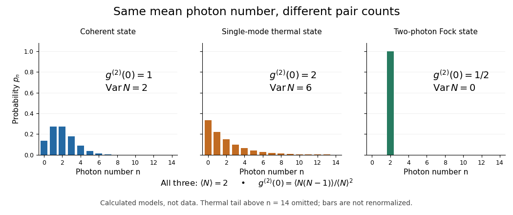
For a single mode in thermal equilibrium, its quantum harmonic oscillator energy ladder gives a geometric distributionIts probability generating function is $F(z)=(1-q)/(1-qz)$. Differentiating twice gives $F^{\prime \prime }(1)=2q^2/(1-q{)}^2=2{\mu }^2$, hence $g^{(2)}(0)=2$. At the chosen mean $\mu =2$, $q=2/3$, $p_0=1/3$, $p_1=2/9$, $p_2=4/27$, and $\mathrm{Var}N=6$. Rare high occupations increase the pair count even though the mean matches the other preparations. The geometric weights also arise from a Gaussian mixture of coherent states.^[ref]

Single-mode selection is essential to this factor of two. If $M$ independent equally populated thermal modes are collected together, let $N={\sum }_{j=1}^M{N}_j$ with $⟨N_j⟩=\mu /M$. Adding their variances gives $\mathrm{Var}N=\mu +{\mu }^2/M$, hence $g^{(2)}(0)=1+1/M$. Averaging over many unresolved modes can make thermal pair counts approach the independent-count reference.

For a coherent state, write $a|\alpha ⟩=\alpha |\alpha ⟩$ and $|\alpha ⟩={\sum }_n{c}_n|n⟩$ in number states. The annihilation operator gives $c_{n+1}\sqrt{n+1}=\alpha c_n$, so $c_n=c_0{\alpha }^n/\sqrt{n!}$. Normalization yields $|c_0{|}^2=e^{-|\alpha {|}^2}$. Thus photon statistics follows a Poisson distribution with $\mu =|\alpha {|}^2$, and the normal ordering of every moment gives $⟨(a^{†}{)}^k{a}^k⟩={\mu }^k$. This factorization is the defining virtue of coherent states for optical calculations.^[ref]

As an original comparison, choose $\mu =2$. Then $p_0=e^{-2}$, $p_1=p_2=2e^{-2}$, $\mathrm{Var}N=2$, and $⟨N(N-1)⟩=4$. A two-photon Fock state also has mean two but has $\mathrm{Var}N=0$ and pair moment two. ConsequentlyIn particular, $|1⟩$ cannot supply a pair. Nevertheless, photon statistics alone does not determine a quantum state: averaging $|\alpha ⟩⟨\alpha |$ over a uniform quantum phase removes its off-diagonal entries while retaining exactly the same $p_n$ and these equal-time moments.

Independent loss alone leaves normalized factorial moments invariant: if every input photon is retained with probability $\eta$, binomial thinning conditional on a total gives $⟨K⟩=\eta \mu$ and $⟨K(K-1)⟩={\eta }^2⟨N(N-1)⟩$. Both powers cancel from $g^{(2)}(0)$. Fewer coincidences still mean poorer statistical precision.

Now let each channel contain a signal rate $s_i$ and an independent Poisson process background rate $b_i$, independent also of the signal. Put ${\rho }_i=s_i/(s_i+b_i)$. The pair density is $s_1{s}_2{g}_{\mathrm{sig}}^{(2)}+s_1{b}_2+b_1{s}_2+b_1{b}_2$. Dividing by $(s_1+b_1)(s_2+b_2)$ proves the displayed formula, for the same bin and timing response. For chosen equal signal fractions ${\rho }_1={\rho }_2=4/5$, ideal signal values $0,1,2$ become $9/25,1,41/25$. Background pulls both dips and peaks toward one.

This calculation assumes additive, mutually independent background counts. Scattered coherent light that interferes with the signal, correlated electronic noise, or recovery effects require a different model. Correcting a dip without independently estimating the backgrounds cannot establish photon antibunching.

For stationary continuous detection, let $C_j$ count all cross-channel pairs with $t_2-t_1$ in a bin of full width $\Delta \tau$, and let $r_1,r_2$ be observed single-count rates. Let $T_j$ be their joint live observation time at that delay, approximately the common duration $T_{\mathrm{obs}}$ when delays are short. Independent streams have expected pair count $r_1{r}_2{T}_j\Delta \tau$, giving the displayed estimator. It estimates a bin average of second-order optical coherence, further blurred by detector timing response. For a finite uninterrupted run the exact overlap weighting is $T_{\mathrm{obs}}-|\tau |$ inside the delay integral, rather than a constant at long delays.

For an original numerical example, choose $r_1=2000{\mathrm{s}}^{-1}$, $r_2=3000{\mathrm{s}}^{-1}$, $T_j=100\mathrm{s}$, and $\Delta \tau =10\mathrm{ns}$. The independent reference is six pairs per bin. Chosen counts $C_j=3,6,12$ give estimates $0.5,1,2$; they are teaching inputs with large counting fluctuations, not historical measurements. For pulsed sources, compare properly normalized same-pulse and separate-pulse coincidences instead of assuming this continuous-source baseline.

Detector dead time suppresses nearby same-detector counts and can manufacture an apparent dip in a single-detector record. Two independent detector channels avoid that particular same-channel exclusion, but shared electronics can still reject pairs. Timing spread and wide bins wash out narrow features. A device recording only the first stop after each start measures a waiting-time distribution; interpreting it as all-pair correlations requires a sufficiently low stop probability over the relevant delay range.

The photoelectric effect is the release of electrons from matter following photon absorption. Here the focus is emission from a metal surface into vacuum: a photon supplies energy, the work function pays the escape cost, and the remainder can become the emitted electron's kinetic energy. A photocurrent counts collected electric charge; a stopping potential probes the upper kinetic energy limit. These are different measurements.

In 1905, Albert Einstein proposed that an individual light quantum could transfer its whole energy to one electron. His §8 allowed losses before escape, distinguished the fastest emitted electrons from the rest, and predicted a straight stopping potential versus frequency relation with a material-independent slope. He separately predicted that changing light intensity changes the number emitted without changing their velocity distribution under otherwise identical conditions. He also discussed incomplete transfer and limits to the account.^[ref]

The useful modern starting model is a clean, homogeneous metal with independent single-photon events, negligible initial thermal broadening, negligible lowering of the surface barrier by an applied electric field, and negligible electric fields from the emitted electrons themselves. Specify the surface and its work function; it is not enough to name the bulk material. The Einstein photoelectric equation describes the upper edge of the emission energy distribution. It neither predicts that every absorbed photon liberates an electron nor supplies the whole photocurrent curve. Its appeal is that a complicated surface process still exposes the universal Planck constant through a simple slope.

The photovoltaic effect is the production of an electric potential difference or an electric current by photon absorption in a material or device. In a semiconductor, absorbed photons generate electrons and electron holes; asymmetric transport and selective collection can maintain distinct quasi-Fermi levels and deliver electrical power to a load. An equilibrium built-in potential alone supplies no continuous electrical power.