
Mitochondrial oxygen electrode assay 2026-10-18
In Respiratory enzymes in oxidative phosphorylation. I. Kinetics of oxygen utilization (1955), Britton Chance and G. R. Williams examined isolated liver mitochondria in isotonic medium with substrate and inorganic phosphate. A one-millilitre optical cuvette held the suspension. A vibrating platinum electrode lay outside the light path; calibrated electric current followed dissolved oxygen, with rapid changes recorded by a galvanometer oscillograph. Air-saturated and oxygen-depleted readings checked sensitivity. Their Figure 2 shows ADP additions accelerating oxygen consumption, followed by return to slow respiration; repeated additions restored acceleration. Figure 4B compares delayed substrate addition after ADP incubation with the reverse order, supporting little unrelated ADP loss in that preparation. These comparisons support coupling to ADP utilization. The authors discuss dilution, sensitivity changes and atmospheric oxygen entry, which especially biases slow respiration. The readout did not directly measure the membrane potential or prove the later chemiosmosis mechanism.[ref]
Respiratory enzymes in oxidative phosphorylation. I. Kinetics of oxygen utilization by Britton Chance and G. R. Williams. pp. 383–386, Preparations and Method, Figures 1–2; pp. 387–389, Endogenous Substrate and Figure 4B; Figure 5: rapid recording
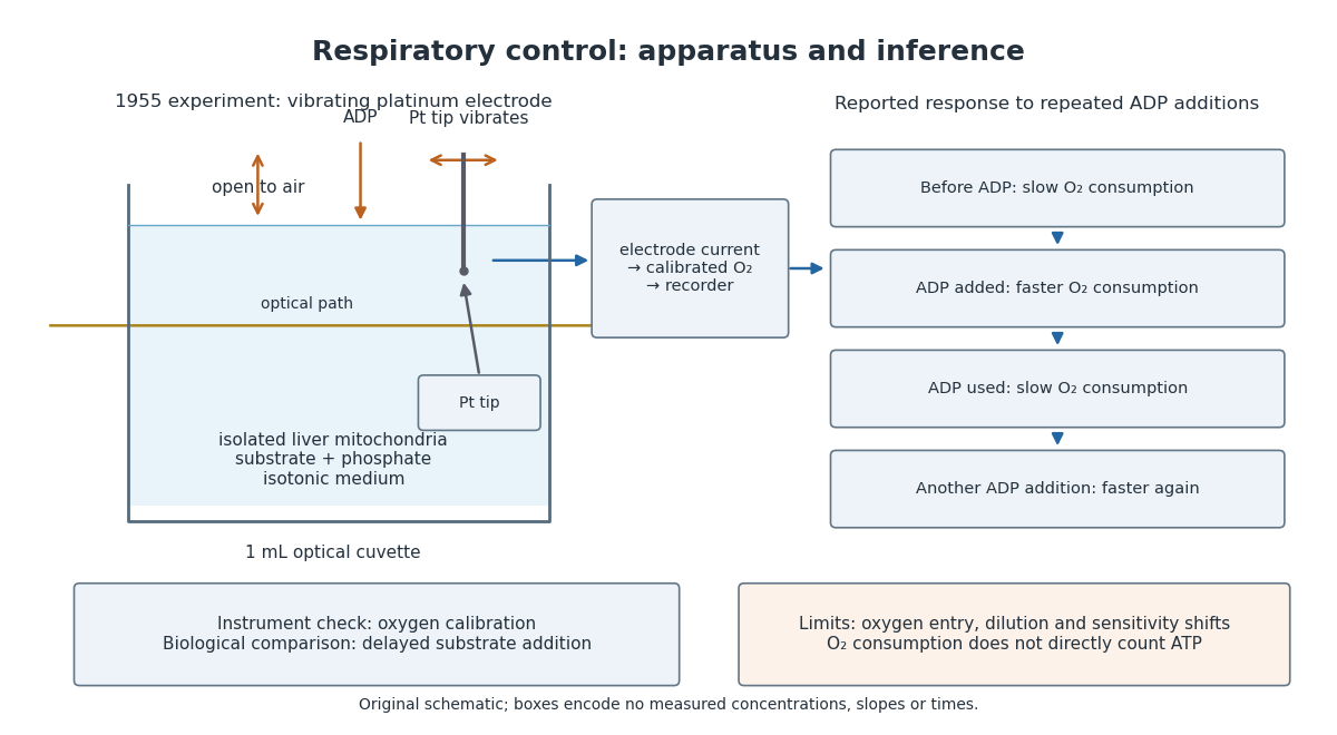
A control can test either the instrument or the biology. Calibrating electric current against oxygen checks the former; comparing responses before and after an ADP addition checks the latter. A valid calibration cannot by itself establish ATP formation, and a repeatable biological response cannot by itself fix an instrument's sensitivity.
Near a renormalization-group fixed point, expand a difference between two nearby models in eigenvectors of the stability matrix. An irrelevant operator direction has , so its dimensionless coefficient shrinks under increasing length factor . A relevant operator direction grows and must be tuned to study the same critical behavior. This is a mechanism for losing microscopic detail, not an assertion that every parameter disappears. Critical temperature, individual amplitudes and regular contributions to free energy can remain material dependent.
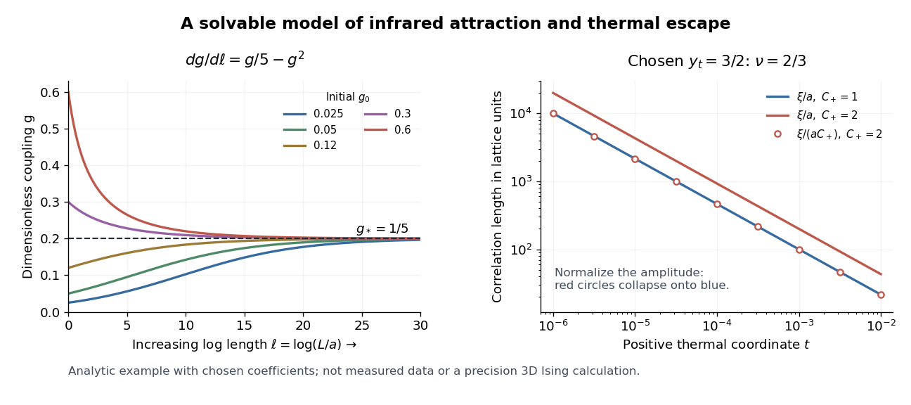
For the solvable example, write . Its exact solution gives . At the thermal stopping scale this is of order . If the stopped correlation length is smooth in , the leading correction to its power law has that order. Thus two microscopic couplings can yield the same limiting critical exponent, yet approach it at different rates.
This mechanism makes universality useful: one tractable representative can predict critical exponents and normalized scaling forms for many systems in its universality class. A liquid-gas critical point and a scalar magnetic transition can share a long-distance description even though their microscopic constituents differ. The scope must be checked: spatial dimension, order parameter symmetry, interaction range, and extra soft variables can change the renormalization-group fixed point.
In his lecture, Kenneth Geddes Wilson connects limiting renormalization-group fixed points with common critical behavior and states the limits of his elementary truncation.[ref]
The Renormalization Group and Critical Phenomena by Kenneth Geddes Wilson. Section II, pp. 110–112: truncation limits and common critical behavior
Add a thermal scaling coordinate , with its critical value subtracted, satisfyingThis is a relevant direction of a fixed point. A thermal scaling coordinate agrees to leading order with a nonzero multiple of reduced temperature; in a general model it can mix several bare parameters. An ordering conjugate field is held at its critical value. The combined stability matrix at has eigenvalues and . Attraction along therefore does not make the critical point attractive against thermal detuning. The critical surface in this example is .
Let denote the correlation length in microscopic lattice units. A renormalization-group transformation of length factor givesIndeed, a tail with exponential envelope becomes under . Choose the stopping scale so that the transformed thermal coordinate is or . If the stopped correlation length tends to a finite nonzero value as the irrelevant coupling approaches , thenThe limit requires and enough room between , , and the sample size. Singular dependence on a dangerously irrelevant coupling or a marginal operator needs separate analysis. On an ordered branch, use the connected correlation function in a pure thermodynamic phase.
For a completely specified illustrative scaling model choose and for . Then gives , whereas gives . With , and . Models with and have different lengths but identical curves after plotting against . This collapse checks the chosen scaling law; agreement of real data would test that law, rather than follow from this example. Neither nor is being fitted to a three-dimensional Ising model.
A solvable infrared renormalization flow 2026-10-18
Take the following bounded analytic example for a dimensionless positive coupling , with fixed and :Increasing means increasing observation length , hence motion toward the infrared fixed point. This convention matters: if the inverse-length scale is , the same trajectory has renormalization-group beta function . The two derivatives have opposite signs.
To solve the equation, set . It obeys , a linear ordinary differential equation. ThereforeFor its denominator is positive, and stays between and . Thus the trajectory is bounded on this domain. The renormalization-group fixed points are and . The derivative of the length-flow right-hand side is : zero is repulsive from positive , whereas has eigenvalue and attracts positive trajectories. Linearization gives near . The inverse-length beta function has positive derivative at the same infrared-attractive point.
For the chosen , take two starting models with and . At , , so their couplings are respectively and . Both move toward , from opposite sides. They are still visibly different: slow decay of an irrelevant operator can leave substantial corrections at accessible lengths. The case stays exactly zero and is outside this positive-coupling basin.
Use a dimensionless statistical Hamiltonian , so that the partition function is . Choose a normalized blocking kernel with . For the majority example it is one when every block has its prescribed majority, and zero otherwise. Define the coarse statistical Hamiltonian by the displayed sum. Then an elementary interchange of finite sums provesThe probability of a retained pattern is therefore its original marginal probability. For any observable of the retained variables,This is the sense in which elimination preserves predictions for retained information. It does not reconstruct every microscopic observable from a block sign.
Next express positions in units of the enlarged spacing: , where . In a continuum version, rescale the retained scalar field as well to restore a chosen gradient energy coefficient; any change in the integration measure contributes to the field-independent term. The result is a new set of dimensionless couplings. Repeating the procedure defines a renormalization-group flow. Additional interactions and the additive constant generally appear, even if the starting statistical Hamiltonian was simple. Keeping only a few terms is an approximation; the equality of partition functions above applies to the complete coarse weight. See also the Wilsonian coarse-grained statistical Hamiltonian for integration over fast Fourier modes.
Block-spin coarse-graining 2026-10-18
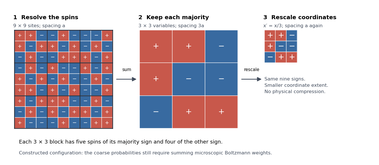
Consider Ising spins on a square lattice of spacing . Divide it into disjoint blocks and retain the majority sign . Each block contains nine spins, so a tie is impossible. For example, five positive and four negative spins produce . All configurations are assigned a retained sign; the individual pattern within a block is lost. A coarse-grained variable has fewer possible values than the microscopic configuration it summarizes.
The spacing between block centres is . In coordinates it is again , so the retained pattern can be compared with the original lattice at the same numerical cutoff. This coordinate change does not physically shrink the sample. A majority picture alone does not specify the new interactions: the blocking kernel and original Boltzmann weights determine their probabilities. The figure is a constructed configuration, not a simulated equilibrium state or a claim that majority blocking closes the nearest-neighbour Ising model.


Renormalization of spontaneously broken gauge theories Created 2026-10-18 Updated 2026-10-25
Renormalization of spontaneously broken gauge theories means that the Higgs mechanism can generate gauge boson masses while a fixed finite set of renormalized couplings, masses and field normalizations still suffices to absorb ultraviolet divergences. The symmetry constrains the counterterms even when the chosen vacuum expectation value hides it. This makes radiative corrections to the electroweak interaction calculable after inputs have been fixed by renormalization conditions.
A useful distinction is between choosing variables that display the physical particles and choosing variables that display good power counting. Unitary gauge removes the would-be Goldstone bosons from the explicit fields. R-xi gauge keeps them and the required Faddeev-Popov ghosts in intermediate Feynman diagrams, exposing simpler large-momentum behavior. The physical scattering amplitude must agree after all contributions and counterterms have been included consistently.
In Renormalizable Lagrangians for massive Yang-Mills fields (1971), Gerard 't Hooft constructed spontaneously broken gauge theories with massive gauge bosons. His worked SU(2) gauge theory with an adjoint Higgs field leaves a massless photon; it is a demonstration model, not the full chiral Standard Model. The gauge fixing, Faddeev-Popov ghosts and Ward identities connect renormalizability with physical unitarity.[ref]
Renormalizable Lagrangians for massive Yang-Mills fields by Gerardus 't Hooft. §§3–5, pp. 171–177; Eqs. (3.8)–(3.14)
Regularization and renormalization of gauge fields (1972), by Gerard 't Hooft and Martinus J. G. Veltman, developed dimensional regularization with recursive subtraction of ultraviolet subdivergences. It continued Feynman integrals in the dimension, keeping the relevant Ward identities in non-anomalous cases; its final section examined quantum anomalies. The procedure does not make an inconsistent chiral gauge theory consistent: gauge anomaly cancellation remains essential.[ref]
Regularization and renormalization of gauge fields by Gerardus 't Hooft and Martinus Justinus Godefridus Veltman. §1, pp. 189–191; §4, pp. 198–205; §6, pp. 206–208
The organizing proof outline is to use good large-momentum propagators, subtract every divergent subgraph, and constrain the remaining local divergences by the Ward identities. A finite family of allowed counterterms must close under this operation at every loop order. The same identities must remove unphysical intermediate contributions from physical amplitudes. Power counting alone establishes neither closure nor these cancellations. Modern BRST symmetry packages these restrictions; the scalar subtraction below illustrates only locality.
Carnot refrigerator Created 2026-10-18 Updated 2026-11-05
A Carnot refrigerator runs a reversible Carnot cycle in the direction that removes heat from a cold reservoir at and delivers to a hot reservoir at . It requires supplied work . Zero total entropy production gives .
Its coefficient of performance, defined as useful cooling divided by supplied work, is thereforeAll temperatures here are absolute. The ratio can exceed one because supplied work moves heat rather than being the only energy delivered to the cold-side process. For reservoirs at and , the reversible value is five. A real refrigerator produces entropy and requires more work for the same cooling between those reservoirs. The ideal result is a limit, not a claim of finite cooling power without thermal gradients.
Abbé refractometer Created 2026-10-18 Updated 2026-11-05
An Abbé refractometer places a small sample between an illuminating prism and a measuring prism, then locates the boundary between bright and dark parts of an angular field. That limiting ray determines the sample's refractive index through Snell's law and the known measuring-prism geometry.
The prism surfaces must be clean and the sample must make good optical contact: a trapped air layer introduces a different interface. Because refractive index varies with wavelength and temperature, a useful reading specifies both; an instrument using white illumination needs compensation for the colored boundary caused by dispersion. A reference liquid checks the reading before an unknown sample is measured.
Prism minimum-deviation index measurement 2026-10-18
A prism minimum-deviation index measurement infers a transparent sample's relative refractive index from two angles: its known apex angle and the smallest deviation of a selected spectral line. A spectrometer combines a source and slit, a collimator, a rotating optical prism table, and a viewing optical telescope with an angular readout. The collimator supplies a nearly parallel beam; the optical telescope locates its emergent direction. This turns an otherwise difficult measurement of the phase velocity of light into a measurement of angles.
For the symmetric path through a uniform optical prism, with the same external medium at both faces and positive refractive indices,The angles are measured from face normals. This is the minimum deviation relation, not a formula for an arbitrary prism orientation. An absolute refractive index additionally requires .
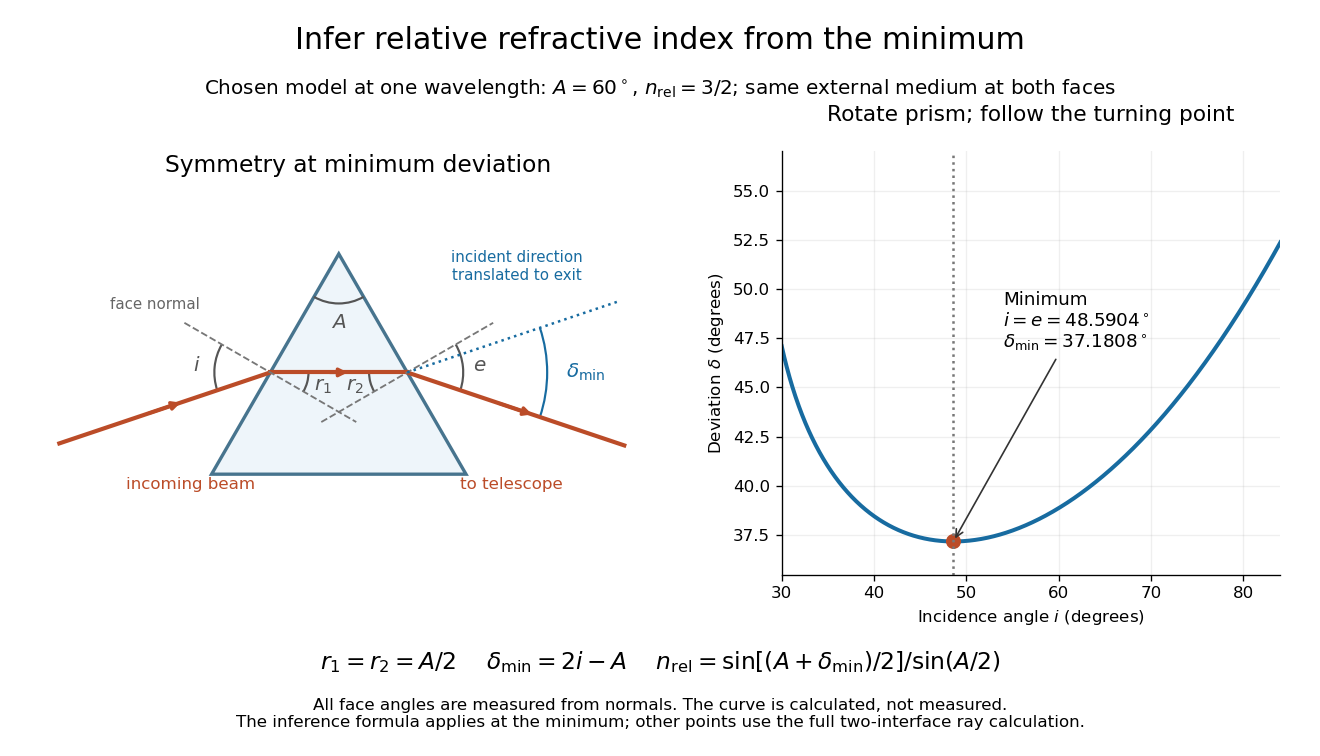
Prism minimum-deviation index measurement: symmetric ray geometry and an independently calculated deviation minimum
. The original model chooses and at one fixed wavelength. The left panel marks face normals, equal internal angles, apex angle and deviation from the undeflected incident direction. The right panel calculates deviation versus incidence from two applications of Snell's law; the marked minimum is the only orientation used for the index inference. No points are experimental observations. Details.
For example, stipulate and . Then and . Substitution recovers . These synthetic values illustrate the geometry; they are not readings for the prism in the laboratory protocol below.
A Michigan State University teaching experiment uses a mercury lamp, slit, collimator, prism table and optical telescope, with a subsidiary angular scale read to one arcminute. First focus the optical telescope on a distant object; with the prism removed, align its crosshair to a narrow vertical slit image, focus the collimator, and establish the direct-beam zero. Insert and centre the prism. Select the green mercury spectral line, tabulated at , then rotate the prism while tracking its image with the optical telescope. Locate the turning point where continued prism rotation reverses the image motion, and read the deviation. Re-establish the minimum separately for each other spectral line. The protocol assumes ; that assumed apex angle is not an independently measured result. [ref]
The Prism Spectrometer. introductory-physics-experiments-physics-252-version-4-0-michigan-state-university; Michigan State University, The Prism Spectrometer, Physics 252 v4.0: pp. 2, 5–9; apparatus, vernier readout, alignment, turning point and wavelength table
For an uncertainty-aware implementation, repeat the turning-point search from both prism-rotation directions, recheck the direct-beam reference, and record individual readings before averaging. Independently determine or include its calibration uncertainty; record the chosen spectral line, sample identity, temperature and surrounding-air conditions. These are proposed controls deduced from the inference, not claimed additional instructions or results of that manual. Finite slit width, unresolved spectral lines, imperfect collimation, table tilt, angular calibration and sample nonuniformity can limit the inferred refractive index. One arcminute readout resolution alone does not establish one arcminute total measurement uncertainty. A single selected wavelength gives one index, not a measured optical dispersion curve.
A short geometric derivation uses and . Reversibility exchanges entrance and exit. At the symmetric stationary path, and ; applying Snell's law gives the displayed index relation. The plotted calculation checks that this stationary point is a minimum on the chosen transmitting branch. To assess local sensitivity, differentiate the inferred index using angles in radians:This first-order relation exposes both angular contributions; it is not an instruction to add signed systematic errors as independent random errors. In the synthetic example, a deviation error of arcminute at fixed changes the inferred relative refractive index by approximately .
For a uniform linear medium with isotropy and local constitutive response, Maxwell equations give . Here is permittivity and is magnetic permeability. Since , the relative permittivity and the relative magnetic permeability obeyIf both responses are real and positive with negligible loss, and the ordinary positive-index branch is intended, then . If additionally , then . All these responses must be evaluated at the electromagnetic wave's frequency; a static relative permittivity cannot simply be substituted at an optical frequency. [ref]
Refractive index. RP Photonics Encyclopedia by Rüdiger Paschotta; What is a Refractive Index?: squared constitutive relation and frequency-specific material responses
With loss, use a complex index and explicitly fix the phase convention for complex amplitudes. For with , its wave amplitude has factor . A forward attenuating branch has , while its wave phase is controlled by . The complex relation alone leaves a choice of sign: the physical solution also needs causality and the appropriate radiation or decay condition. In negative-index media the physically selected real part can be negative. The positive square root is therefore not a universal rule for complex or negative-index media. Direction and polarization of an electromagnetic wave also matter in a plane wave in an anisotropic dielectric, for which one scalar index need not describe every propagation branch.
Refractive index and wavelength 2026-10-18
For a linear stationary interface, phase matching at a planar wave interface preserves frequency: the incident and transmitted electric fields must oscillate together at each boundary point. Their phase velocities can differ, so their wavelengths differ. Writing , the definitions giveThis explains the compressed wavefront spacing in the figure without changing the time between crests at the interface. Moving interfaces or time-dependent material responses need not preserve frequency. [ref]
Chapter 31: The Origin of the Refractive Index. The Feynman Lectures on Physics, Volume I, §31–1: boundary oscillations, vacuum and medium wavelengths, Fig. 31–2
The notation labels refractive index by vacuum wavelength; it does not mean the wavelength inside the material. Dependence on , equivalently on frequency, is optical dispersion. The field driving the material induces oscillating electric charges; their emitted electromagnetic fields combine with the applied field to change the resulting wave phase. This collective response motivates refractive index, rather than a picture of independently delayed little pieces of light. [ref]
Chapter 31: The Origin of the Refractive Index. The Feynman Lectures on Physics, Volume I by Richard Feynman and others; §31–1: superposition of the applied field and fields from driven charges; near-unity-index approximation
To distinguish three speeds, track a wavefront for phase velocity, a narrow wave envelope for group velocity, and the earliest newly introduced disturbance for front velocity. For a transparent differentiable propagation branch,The denominator is the group refractive index. It describes envelope transit when loss and reshaping are small. It need not equal , and neither phase velocity nor a reshaped pulse peak generally measures signal arrival. The front velocity article explains the separate relativistic causality constraint and why a detector threshold is not an exact causal-front measurement.
Relative refractive index 2026-10-18
The relative refractive index of medium two with respect to medium one is , using their absolute refractive indices at the same frequency. For transparent media with isotropy and positive refractive indices, Snell's law gives , with the angles measured from the interface normal. Thus a refraction measurement in air directly determines an index relative to air. Converting it to an absolute refractive index requires the refractive index of that air; replacing it by one is an approximation.
Complex refractive index Created 2026-10-18 Updated 2026-10-20
For a plane wave proportional to , the complex refractive index separates phase propagation from attenuation. In a nonmagnetic medium , so and . The passive branch has . If and , then and . These signs assume the convention for the complex permittivity.
Slotted-line waveguide measurement 2026-10-18
MIT's documented slotted-line waveguide measurement shorts one end of a rectangular electromagnetic waveguide and excites it through a probe coupled by capacitance. A second such probe moves through a longitudinal slot, aligned with the wall electric current to reduce disturbance. Its output locates axial standing wave nulls. The book's standing-wave setup chooses a frequency above the first waveguide cutoff frequency and below higher-mode cutoffs. Lowering it below the first cutoff instead reveals spatial decay away from the source. The text supplies apparatus and an observable comparison, rather than a table of measured null positions.[ref]
The inference can be checked without assuming that detector output is proportional to electric field amplitude. At fixed measured frequency, record several minima at coordinates ; then estimate when the minima are consecutive. This uses positions alone. Compare the result with the guided wavelength prediction using independently measured and . The spacing above is a synthetic example, not a reading from the MIT apparatus.
Additional proposed controls are to keep probe insertion fixed, repeat the scan in both directions, recheck source frequency, and compare shallow probe settings for shifts in the minima. These test probe loading, mechanical backlash and drift. A deliberately reflecting termination supplies the standing wave; varying its position should translate the pattern without changing adjacent-null spacing in a uniform single-mode region. Source-adjacent evanescent waves, unintended reflections, additional propagating normal modes, detector noise and finite positional resolution can spoil that inference. A disappearing remote signal alone does not distinguish below-cutoff decay from loss or poor excitation, and a scan at one frequency does not measure a pulse's group velocity.
Guided wavelength 2026-10-18
The guided wavelength is the distance for a change of axial wave phase in a propagating normal mode. For the vacuum-filled rectangular electromagnetic waveguide,for , with and . It exceeds the vacuum wavelength at the same frequency. This longer axial spacing is consistent with : multiplying by gives the phase velocity, not the group velocity.
Two oppositely traveling fields at the same frequency form a standing wave. For a perfect electric short at , the total electric field is proportional to , so successive axial electric nodes are separated byThus neighboring minima in a slotted line scan give half a guided wavelength. In the original , example, implies , not . Combined with the chosen , the inferred broad dimension is . Below cutoff, is imaginary and is not a physical periodic spacing.
In a hollow rectangular electromagnetic waveguide with perfect conductor walls and axis , a transverse magnetic polarization has and a nonzero longitudinal electric field . The wall boundary conditions impose around the transverse rectangle. Separation of variables therefore gives , with . Setting either index to zero makes the entire field vanish. Thus there is no or branch. The transverse eigenvalue is , with dispersion relation . This exclusion is specific to this geometry and these boundary conditions.
RC low-pass laboratory 2026-10-18
The University of Colorado Boulder's Lab 3: Filters, §§7.1–7.4, specifies measuring the resistor and capacitor, then driving the assembled RC low-pass filter with a function generator. A two-channel oscilloscope reads actual input and output using high electrical impedance. Sweep the frequency, record the voltage amplitude ratio, and locate . A control compares a cable with a oscilloscope probe on a resistive voltage divider, isolating measurement capacitance before using the probe for the filter. A slow square wave then lets discharge timing estimate the time constant independently. Agreement supports the RC low-pass frequency response; source output impedance, probe loading, and instrument signal bandwidth limit it. These are prescribed measurements, with no measured dataset supplied here.[ref]
The two-channel setup can also test the predicted phase difference directly: for positive frequency , measure the output's time lag between corresponding features of the two sinusoids. For this single-stage model the phase lies between and , so choose the lag within a quarter cycle and calculate . At the cutoff frequency the predicted lag is one eighth of a cycle. This tests the timing part of the frequency response as well as the voltage ratio.
RC low-pass output loading 2026-10-18
A real electrical load can draw electric current from the output. For a load resistor across the capacitor, Kirchhoff's current law instead givesTherefore the loaded continuous-time frequency response isLoading reduces the eventual gain and shortens the time constant. With the constructed values and , , , and the corner relative to the loaded low-frequency gain moves to . A step now approaches . A quicker rise alone would conceal the error in the final voltage.
With the ideal input voltage source set to zero, the output impedance seen by the electrical load isThis follows from Thévenin's theorem: the resistor and capacitor are then in parallel. A sufficient small-loading condition is over the frequencies of interest. An oscilloscope is itself an electrical load: its input electrical resistance and cable or probe capacitance can both change the response. Pure extra parallel capacitance increases and lowers the corner, whereas a finite parallel electrical resistance gives the different gain-and-corner changes above.
The definition of input also matters. If voltage is prescribed inside a source with series electrical resistance , the unloaded response to that internal source uses . If the actual voltage at the filter input terminal is measured, the ratio of output to that measured input still uses . Measuring both terminals avoids mistaking a source setting for the voltage delivered to the filter.
RC low-pass step response 2026-10-18
The step response describes a sudden persistent input change. Suppose the input becomes a constant at , and the initial capacitor voltage is . Finite electric current leaves that voltage continuous. Subtract from the RC low-pass filter equation: the remaining error satisfies . Separating variables givesFor an initially uncharged capacitor and a to step in the constructed example,At one time constant, , the voltage is , about of its final value. The voltage error then continues its exponential decay. This is different from a pure delay: the output starts changing immediately, yet takes time to approach the target.
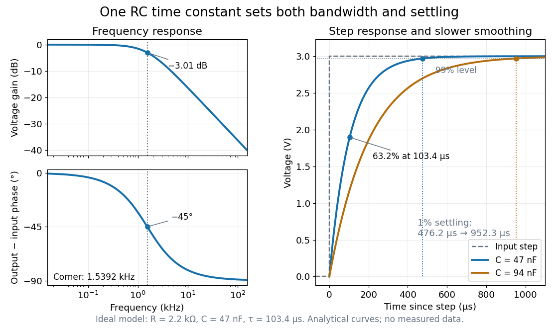

Define settling time relative to the total voltage change: require thereafter, with . The exponential decay is monotone, soFor settling, ; the to rise takes . Reducing the cutoff frequency by doubling doubles both times. This reciprocal relation is the useful connection between signal bandwidth and response speed: stronger suppression of rapid noise comes with slower tracking of wanted changes.
There are unlisted articles, also show them or only show them.