
Active-pixel sensor 2026-10-18
Bolometer 2026-10-18
A bolometer detects absorbed electromagnetic radiation through the resulting change in temperature, often read as a change in electrical resistance. Its response depends on absorbed power, so interpreting an optical spectrum requires accounting for the incident wavelength band and detector calibration.
Vacuum photodiode Created 2026-10-18 Updated 2026-10-20
Phosphoenolpyruvate 2026-10-18
Phosphoenolpyruvate supplies a phosphate group to ADP in the final glycolysis step catalyzed by pyruvate kinase. The free ionic form used in the worked balance has charge .
Work by Philip E. Stewart 2026-10-18
Vaporization 2026-10-18
Vaporization changes a liquid into a gas. It includes evaporation at a surface and boiling within the liquid. Below the liquid-gas critical point, equilibrium conversion along the liquid-vapour phase coexistence curve involves latent heat; the liquid and vapour have equal chemical potential there.
Condensation Created 2026-10-18 Updated 2026-11-05
Condensation is conversion of a vapor into a liquid. Cooling vapor-bearing air below its dew point is a familiar example: droplets form on a cold surface as the saturation vapor pressure falls. In a mixture, the relevant comparison uses the condensable component's partial pressure, rather than the mixture's total pressure alone.
Creating a new droplet costs interfacial free energy, while conversion to the stable liquid lowers bulk free energy. A nucleation barrier can therefore permit supersaturated vapor before droplets appear. A pre-existing surface can lower that barrier through heterogeneous nucleation. Condensation also releases latent heat, so a cold plate or condenser must remove heat as liquid accumulates. At vapor-liquid equilibrium, evaporation and condensation continue microscopically with equal average opposing rates.
Liquefaction of gases Created 2026-10-18 Updated 2026-11-05
Liquefaction converts a gas into a liquid. For a pure substance below its liquid-gas critical point, compression can cross the liquid–vapor coexistence boundary; cooling can also bring a vapor to its saturation condition. Above the critical temperature, pressure alone does not produce a distinct liquid–vapor transition.
A practical cycle removes compression heat and cools the gas before collecting the liquid. The Joule-Thomson effect can provide cooling during expansion in the appropriate regime, but its sign depends on the gas and operating conditions. The collected liquid releases latent heat as it forms, so sustained production requires continued heat removal. These requirements explain why a high-pressure vessel alone is not a general liquefier.
Metal-insulator transition Created 2026-10-18 Updated 2026-10-20
A change between a material behaving as an electrical conductor and as an electrical insulator. The distinction concerns the limiting electronic response as temperature tends to zero; finite thermally activated electrical conductivity alone does not establish a metallic state. A Peierls transition opens a band gap through a change in the crystal structure.
Digital optical phase conjugation 2026-10-18
Digital optical phase conjugation uses a wavefront sensor and a spatial light modulator to measure an incident field and launch a beam with the opposite spatial wave phase. A phase-only spatial light modulator illuminated uniformly generally does not reproduce the incident wave amplitude as well; exact requires the appropriate wave amplitude and polarization of an electromagnetic wave too. The experimentally useful question is how much of the original optical mode can be recovered with the measured and controlled field components.
In 2010, Meng Cui and Changhuei Yang demonstrated digital optical phase conjugation through a prepared multiple scattering sample. They dried mixed-size polystyrene microspheres on cover glass, added immersion oil, and sealed them with another cover glass. A 532 nm laser supplied signal and reference beams. The signal crossed the sample between two objectives; the reference interfered with it on a charge-coupled device. Phase-stepped wave interference recovered the spatial wave phase; a calibrated spatial light modulator imposed its negative on the reference-derived return beam. The reference supplied playback power, without nonlinear mixing pumps. An optical camera read out the recovered signal. With the same sample and a zero-phase spatial light modulator control, the return instead produced a scattering of light pattern. This comparison supports mode recovery by spatial wave phase control, not merely increased illumination. A separate ordinary-mirror control tested source displacements. Finite sampling and collection limited recovery; the system controlled wave phase rather than the complete vector field. These restrictions distinguish demonstrated reconstruction from exact reversal of every scattered component.[ref]
Model a thin transparent plate by a lossless reciprocal phase screen with transmission at the chosen angular frequency. Both passages multiply the local field by the same : reversing travel does not by itself change the sign of an accumulated optical path length. Assume the plate is stationary, the two passages use corresponding transverse positions, and the plate is adjacent to the return surface or perfectly reimaged onto it. Ignore propagation between these reference surfaces, wave absorption, clipping and intensity-dependent changes. Take the incident boundary envelope to be . Outward transmission gives . Ideal phase conjugation and the second transmission then giveThis is a complete short proof of cancellation in the specified phase screen model. For an ideal ordinary mirror with constant reflection factor , the corresponding envelope is : the extra wave phase is , rather than zero. A constant reflection wave phase changes neither conclusion.
For an original toy optical aberration, let on , take , and chooseThe even term adds symmetric curvature and the odd term makes the two sides unequal. The outward wave phase is ; immediately after ideal phase conjugation it is ; after the second passage it is zero. At , the outward values are , while an ordinary mirror's completed return has values . All wave phases here are unwrapped relative to the central ray and are otherwise equivalent modulo . At a stipulated vacuum wavelength , these outward errors correspond to optical path length errors of . These are chosen values; they are not observations or physical plate thicknesses.
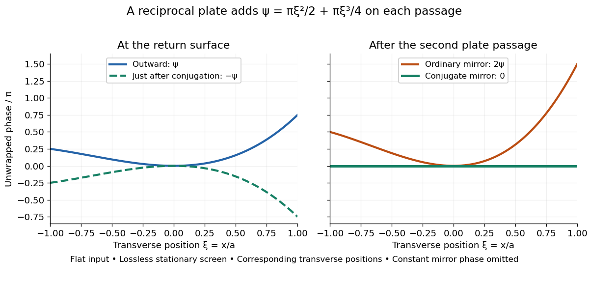
Original thin phase screen example: sign reversal at conjugation and cancellation after the second passage
. Details. 
The wave phase plots make a subtle distinction visible: the field is still curved immediately after phase conjugation, and becomes flat only after crossing the same plate again. More generally, conjugation restores , not a universally flat wavefront. If the plate instead has transmission with real , the return is . Its plate-induced wave phase cancels but its lost wave amplitude does not recover. If the return plate has changed to wave phase , the residual factor is . Those two variations distinguish correction of a stationary optical aberration from universal reversal of loss or material evolution.
Phase-conjugate mirror 2026-10-18
A phase-conjugate mirror is an optical device that implements phase conjugation at its return surface. It may generate the return using an independently supplied beam, as in digital optical phase conjugation; its name specifies the field transformation, rather than a particular reflecting material. Conjugating the transverse complex amplitude and launching the returning longitudinal carrier produces the complete reversed wavevector. A spatially constant leaves the shape of the wavefront unchanged; a spatially varying would add its own wavefront error.
An ordinary flat mirror obeys the law of reflection. At a surface , its reflected plane wave has wavevector , whereas a phase-conjugate mirror returns . Ordinary specular reflection preserves the tangential wavevector. At normal incidence a single plane wave can therefore look identical in the two cases, apart from an overall wave phase and strength; oblique incidence or a curved wavefront reveals the distinction. In boundary-envelope notation an ideal ordinary mirror multiplies the incident complex amplitude by a constant reflection factor , while an ideal phase-conjugate mirror returns its complex conjugate times .
Suppose a calibrated measurement bounds the fractional loss of a nonzero superconducting persistent current by , with , over a duration . Take by choosing the circulation direction. Under the constant-, constant-, undriven RL circuit model,The inequality follows because the logarithm is increasing. The final approximation requires and slightly understates the exact upper bound. If is uncertain, an independently established upper bound on gives the conservative electrical resistance bound. The uncertainty in the initial reading, the final reading, background subtraction and drift must all be included in ; a display resolution alone does not provide it.
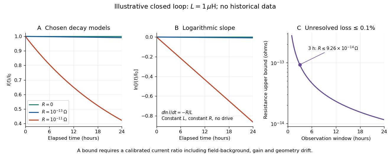
An illustrative exponential decay, its logarithmic slope and the resulting resistance bound
. Chosen numerical model, not historical data: fixed self-inductance and no external drive. The final panel assumes a calibrated fractional-loss bound of at each chosen observation duration. Longer observation tightens the bound only while that fractional uncertainty remains controlled. Details.
For an original illustrative example, let and suppose the corrected electric current ratio after is at least . ThenThese are conditional bounds for stipulated parameters, not values attributed to the 1914 apparatus. With the same but , the model instead gives and : a readily visible loss on the chosen scale.
A resolved decay can be checked using its logarithm:A straight line supports this constant-parameter model; curvature or jumps demand a different account. If an effective electrical resistance varies with time while remains fixed and the loop remains undriven, only its time average is constrained:This does not bound every instantaneous value of . Changing self-inductance or external linked magnetic flux adds terms to the circuit equation, so an uncorrected magnetic signal cannot simply be substituted for . Nonobservation of decay leaves arbitrarily small positive constant electrical resistance compatible with a finite observation: it is not a logical proof that .
Permanganate-iron endpoint and blank model 2026-10-18
The apparatus and motivating measurement are described in permanganate-iron titration; the following is an original account of its possible errors. Assume correct titrant standardization, the acidic permanganate-iron balance, quantitative conversion of the sampled , and additive contributions expressed as equivalent titrant volumes. WriteHere is the sample titre, the titration blank, background reagent consumption, and signed offsets of the observed titration endpoints from the respective stoichiometry conditions after background consumption. The subscripts distinguish sample and blank. is additional sample-specific permanganate demand, absent from the blank; is apparent delivery used to fill an initially air-containing burette tip rather than enter the flask. Assume the blank's tip is already filled; the sample should also have after proper preparation. These terms are a diagnostic model, not measured components of the stipulated blank.
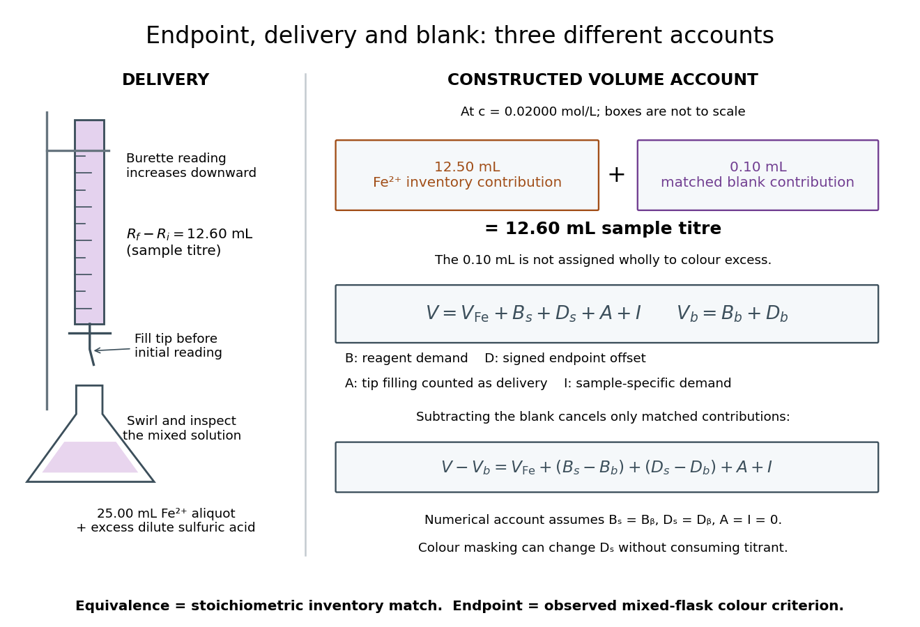

Subtracting the two accounts proves the error relationThe simple inference is valid when this residual is negligible. Matching water and sulfuric acid tests the background terms, but does not by itself establish : flask composition and viewing conditions can differ. A coloured sample can mask residual permanganate, changing the assigned titration endpoint without a corresponding redox consumption. A sample-specific reducing agent instead contributes positive by consuming permanganate. A reagent titration blank cannot measure either effect just by omitting the sample.
A transient purple streak before mixing is not the mixed-flask titration endpoint. Conversely, the equivalence point is the five-to-one inventory match, without a promised visible flag. In the ideal selective model, a persistent excess colour requires some permanganate beyond that match. No particular drop size, waiting time or endpoint offset is stipulated here; the same stated colour criterion must be applied to sample and blank, and its transferability checked.
The model also predicts error direction. If a tip bubble disappears during sample delivery, makes the inferred amount of substance too high because final minus initial burette reading includes liquid that stayed in the tip. Conditioning the tip before the first reading prevents this particular discrepancy; subtracting a separate titration blank is not an instrument repair. Repeated aliquots test scatter, a known added inventory tests the five-to-one response, and an independent titrant standardization tests . These are the proposed controls from permanganate-iron titration, with distinct diagnostic roles; none alone proves absence of all sample interference.
Relativistic dust Created 2026-10-18 Updated 2026-10-25
Relativistic dust is a continuum of noninteracting massive particles with one local four-velocity and negligible pressure. With signature , and rest mass density , its stress-energy tensor has the displayed form. Contracting stress-energy conservation with and using metric compatibility gives . Substituting back yields wherever : each particle follows a geodesic. The cosmological pressureless matter model is a homogeneous application.
Microwave radiometer calibration example 2026-10-18
Consider an original idealized narrow-band model for one matched spatial mode and one polarization of waves. In the classical Rayleigh-Jeans law regime, an available thermal power can be written , where is the effective bandwidth and the equivalent input noise temperature. Assume a linear detector with stable positive gain and absorb its bandwidth, Boltzmann constant and response factor into . Then the output is , with input-referred receiver noise temperature . These are model assumptions, not a reconstruction of the historical electronics.
Two references with known noise temperatures giveso the two-load radiometer calibration yieldsSubtracting the reference equations eliminates the unknown receiver term; substituting back determines it. An arbitrary stable output offset can likewise be eliminated from the interpolation for , although separating that offset from then requires additional information.
For deliberately chosen inputs, set , , and . These are equivalent noise temperatures; physical load thermometry must be converted consistently at the observing frequency. The reference outputs are and . A sky-input output gives . If independent estimates assign to atmosphere, to antenna loss and to ground pickup in this lumped additive model, the residual is .
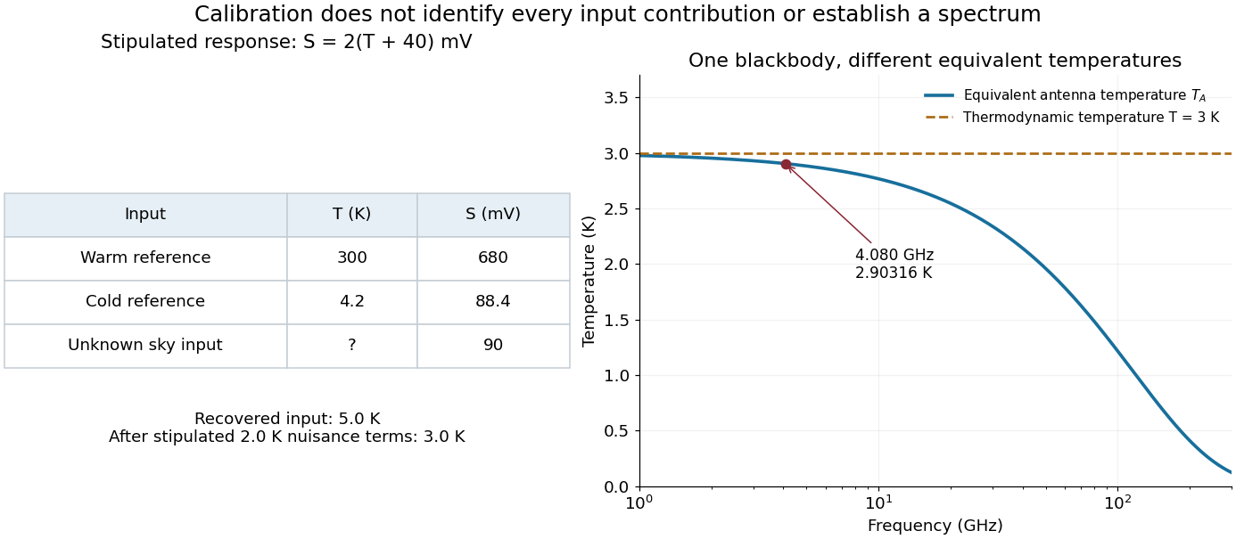
Original calibration arithmetic and the distinction between an antenna temperature and a thermodynamic temperature
. Chosen reference temperatures, receiver response and additive contributions; none are fitted historical measurements. The final panel calculates the Rayleigh-Jeans law equivalent antenna temperature of a stipulated blackbody. A change in frequency changes that equivalent temperature even though the underlying thermodynamic temperature is fixed. Details.
The subtraction exposes what a noise budget must achieve. A error in the assigned atmospheric term becomes a error in the residual, even with exact detector calibration. Multiplicative attenuation requires a different correction: if an isothermal atmosphere has transmission , its ideal contribution is in the same classical equivalent-temperature convention. Recovering then requires both subtracting atmospheric emission and dividing by . The additive toy budget applies when its terms already refer to the same receiver input.
There is also a conditioning issue. If is small, a fixed output error strongly changes the inferred temperature. Widely separated reference temperatures improve the scale determination only if the receiver remains linear over that range; measuring the reference repeatedly tests stability rather than proving linearity. The experiment therefore motivates a model, a calibration and a set of independent checks, each with its own assumptions.
Global causal step in the Penrose theorem 2026-10-18
Assume future null geodesic completeness. The compactness of the future horismos of a trapped surface makes a nonempty compact achronal boundary without edge. Projection along a complete timelike vector field into the Cauchy hypersurface is injective, open by invariance of domain, and closed by compactness. Connectedness forces surjectivity, contradicting the noncompact Cauchy hypersurface. This global step completes the contradiction.[ref]
Gravitational Collapse and Space-Time Singularities by Roger Penrose. p. 59, compactness and noncompactness contradiction
The Null Raychaudhuri equation is the light-ray version of the Raychaudhuri equation associated with Amal Kumar Raychaudhuri. His original work concerned relativistic cosmology.[ref]
Amal Kumar Raychaudhuri by Jayant Vishnu Narlikar. research discussion, PDF pp. 4–6, the 1955 paper Relativistic Cosmology
For the normal null geodesic congruence before its first focal point, null twist vanishes. With an affine parameter , the four-dimensional equation reduces to the displayed ordinary differential equation. The null shear contraction is nonnegative on the transverse screen space, and the null convergence condition makes the other part of nonnegative. Consequently .For , put . ThenA regular negative null expansion therefore cannot persist beyond if the null geodesic extends that far. The null focusing theorem turns this estimate into a focal-point bound. The number refers to an affine parameter, not the proper time of a light ray, which is zero.
For an original soluble model, prescribe constant along one twist-free beam; this does not specify an entire solution of the Einstein field equations. Introduce a positive affine scale and the dimensionless variablesFor an infinitesimal area define before the first zero. Since , where primes now mean , the same model becomesTwo independently checkable solutions areThe nonnegative extra focusing term moves the first zero earlier. Direct substitution into both ordinary differential equations verifies the solutions; numerical integration of the nonlinear equation provides a separate comparison with the linear beam equation.
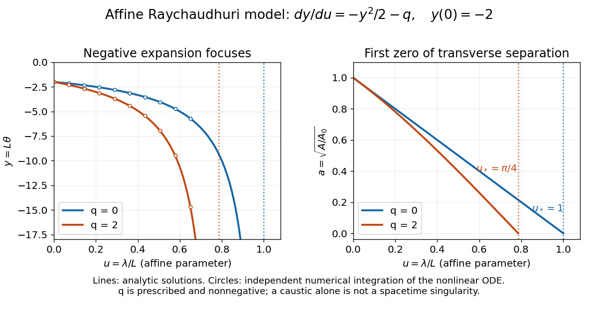
Finite affine focusing in two explicitly defined Raychaudhuri models
. Both beams start with . Curves show the exact solutions for and ; circles independently integrate . The first zeros occur at and , respectively. These are illustrative ordinary differential equation models, not fitted collapse data. Details.
A focal point makes this beam description degenerate, but individual null geodesics may continue smoothly through it. Even converging light in Minkowski spacetime can form a caustic. Converting local focusing into null geodesic incompleteness requires the global step below.
A concrete example separates a trapped surface from a failure of coordinates. Use geometrized units , metric signature , and the regular ingoing Eddington-Finkelstein coordinates of a Schwarzschild black hole with mass :For a round sphere, choose future null vector normalsThe spherical null expansion in ingoing coordinates follows directly from : . At , ; at , it is . Both future light fronts shrink in the second case. At , , so this sphere is marginally outer trapped surface, not a strict trapped surface. In the spherical model this boundary is an event horizon; that identification does not extend to arbitrary geometries.
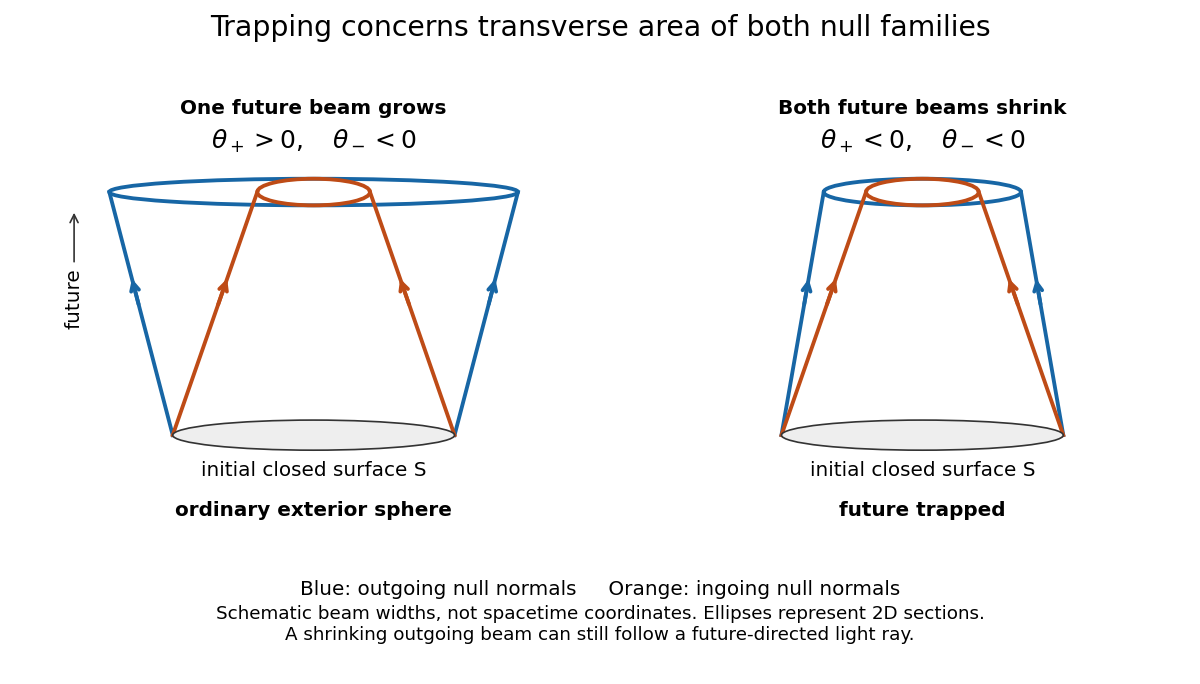
Both future null families contract at a trapped surface
. The schematic compares signs of null expansion. The horizontal separation represents transverse beam width, not a radial spacetime coordinate; the ellipses represent two-dimensional sections. No horizon location or endpoint of a null geodesic is encoded by the drawing. Details.
Although is affine as written, generally obeys . These are valid initial normals for the sign test; use affine rescaling of a null normal before applying the affine Null Raychaudhuri equation. Regularity of the displayed metric tensor at shows why a divergence in another chart would not establish null geodesic incompleteness.
On a compact trapped surface, both null expansions have a uniform negative margin. Sufficiently small smooth perturbations controlling the relevant metric tensor and surface derivatives preserve trapping. This conditional robustness does not prove that every nonspherical gravitational collapse creates a trapped surface.[ref]
Gravitational Collapse and Space-Time Singularities by Roger Penrose. p. 58, small departures from symmetry
Trapped-electron spin-jump readout Created 2026-10-18 Updated 2026-10-20
Hans Georg Dehmelt describes a , Penning trap, with positive ring and negative endcaps apart. Axial RF emission tracked an injected seven-electron bunch losing particles; reducing the drive retained the last electron. A weak magnetic bottle converted spin changes into axial-frequency changes. At successive probe frequencies, counted spin flips traced a resonance.[ref]
Experiments with an isolated subatomic particle at rest by Hans Georg Dehmelt. Dehmelt, pp. 584–589, Figs. 1, 3, 6–7; Columbia scan
The inference can be explained without inventing a detector calibration. Let a weak bottle have on-axis field . The magnetic dipole potential energy adds to the axial harmonic oscillator potential energy, soA change in the magnetic dipole moment therefore shifts the monitored axial angular frequency. This is a simplified readout model, not a quantitative reconstruction of the historical bottle. It illustrates how a transition in one degree of freedom becomes a detectable change in another.
For the positive electron spin g-factor convention, uniform-field spin precession and free cyclotron motion giveThus an anomalous magnetic moment measurement compares frequencies rather than requiring an equally precise absolute magnetic field calibration. The free must first be inferred from trapped motion with the necessary corrections. A spin-flip count versus probe frequency supplies evidence for a transition resonance; it does not directly measure a spatial electron radius. Nor is this radio readout an optical fluorescence record: different experiments require different preparations and detectors. In a precision comparison, repeat scans with changed drive strength and monitor magnetic field drift, motional excitation and detector back-action; these are experimental-design checks, not additional historical observations asserted here.
There are unlisted articles, also show them or only show them.