
RC low-pass frequency response Created 2026-10-18 Updated 2026-10-25
Use the complex amplitude convention , where is the angular frequency and is the frequency in cycles per second. Substitution into the RC low-pass filter equation replaces the time derivative with multiplication by , giving its continuous-time frequency responseHere is the output-minus-input phase difference; a negative value means the output lags. Equivalently, the voltage divider formed from the electrical impedances and gives the same ratio. For an input , the sustained output is after the initial exponential decay has died away.
Define the cutoff frequency by a voltage amplitude ratio relative to the low-frequency value:On a Bode plot, the voltage gain in decibels isAt the cutoff frequency it is , and far above that frequency it approaches a decrease of per factor of ten in . There is a smooth transition rather than an abrupt wall. The squared voltage ratio is one half at the corner; converting that statement to a power ratio requires the same real electrical resistance for the compared voltages. It does not mean that an unloaded capacitor dissipates half the source power.
For and , the cutoff frequency is . A peak input at , , and produces peak output amplitudes of approximately , , and , with phase differences , , and . Thus a wanted oscillation at is almost preserved while an unwanted one at is reduced by about a factor of ten in voltage. The superposition principle lets these two responses be added when both oscillations occur in the same signal.
Work by Raymond S. Castner 2026-10-18
Work by Raymond Rappaport 2026-10-18
Narrow-gap centrifugal stability equation 2026-10-18
For axisymmetric inviscid modes between impermeable cylinders in a thin annulus, let and . The linear azimuthal equation gives and the axial equation gives , where is the kinematic pressure perturbation. Thin-gap incompressibility implies . Eliminating it from the radial equation gives the title equation with . If a plus sign is used for the potential, its coefficient must be defined as , the negative of the usual Rayleigh discriminant.
Fermi contours of an isotropic Rashba band 2026-10-18
For the Rashba effect with , put . If , both Fermi contours belong to the lower branch and bound the singly occupied annulus ; the central disk and exterior are empty. At , the lower occupied disk has outer radius , while the origin is a degenerate point at the Fermi energy. For , the lower Fermi contour has radius and the upper Fermi contour radius . The inner disk has two occupied spin-split eigenstates at each momentum, the intervening annulus has one, and the exterior is empty. Consequently , whereas below the crossing the two lower-branch radii add to . At zero temperature, changing occupation values only on these Fermi contours affects a null set and leaves the integrated carrier density unchanged.
Rashba spin texture 2026-10-18
For with , the lower- and upper-band spinors of unit norm can be chosen asTheir spin expectation values are . They are tangential to circles of constant momentum magnitude, opposite between branches, and reversed at opposite momenta as required by time-reversal symmetry. When , the outer contour belongs to the lower branch and the inner one to the upper branch. For the two Fermi contours both belong to the lower branch and have the same tangential spin orientation at a given angle in polar coordinates. At the Hamiltonian has quantum degeneracy in spin, and no unique spin texture direction is selected.
Ideal binary vapor composition 2026-10-18
For the stipulated A/B ideal solution, put . At the fixed temperature , Raoult's law reduces toThe relative volatility is . For ,Hence every interior vapor-liquid equilibrium pair in this chosen model has A-enriched vapor; neither pure endpoint is enriched. Conversely,For example, corresponds to , and . Equal vapor mole fractions therefore need not mean equal liquid mole fractions.
These are fixed-temperature predictions. During boiling at a specified external pressure, the temperature instead adjusts until . The two stipulated vapor pressures specify only one temperature; they provide no boiling-temperature curve.
Transformation of a random variable 2026-10-18
A measurable function applied to a random variable defines a new random variable . Its probability distribution is the pushforward measure under .
Work by Ramanujan S. Hegde 2026-10-18
Raman spectroscopy 2026-10-18
Raman spectroscopy measures shifted scattering of light to infer internal energy spacings and the molecular response that makes them visible. In a modern illustrative arrangement, narrowband laser illumination replaces the historical arc, an optical filter rejects the strong excitation line, and a spectrograph resolves the weak shifted spectral lines. The illumination, rejection and spectral dispersion are separate jobs. Increasing rejection can conceal small Raman shifts close to the excitation line.
A proposed measurement should record the excitation wavelength, a dark signal, a blank container and the liquid, then compare calibrated line positions and integrated signals under the same collection conditions. Measure optical filter transmission and detector response before using the Thermal Raman line ratio for temperature. Repeat at lower incident power to look for heating or altered sample response. These are suggested checks, not an assertion that the 1928 apparatus implemented modern calibration procedures.
Its appeal is the conversion of internal molecular energy differences into visible spectral lines: changing the excitation can move the whole pattern while preserving characteristic Raman shifts. Combined with vibrational infrared activity, Raman vibrational activity supplies complementary information about molecular vibration. A line pattern can constrain a material's identity or environment, but overlapping bands, fluorescence backgrounds and the finite spectral resolution element prevent an unqualified identification from one peak alone.
Thermal Raman line ratio 2026-10-18
Assume one harmonic normal mode at thermal equilibrium, weak spontaneous excitation far from electronic resonances, the same collection solid angle and wave polarization, and matched response after instrumental correction. The Boltzmann distribution givesHere is the Boltzmann constant, is temperature, and is the probability of vibrational quantum number . Thus . Linear coupling to has squared oscillator matrix elements proportional to for Stokes Raman scattering and for Anti-Stokes Raman scattering. Summing over initial levels gives strengths proportional to and respectively; their ratio is , even when levels above are occupied.
Let and denote line-integrated radiant intensities, meaning power per collection solid angle. The off-resonant electric dipole radiation law adds the fourth power of emitted frequency:The photon rate divides each line's power by its own . Consequently, the ideal response-corrected anti-Stokes/Stokes count-rate ratio has the third power of the same frequency ratio. Peak heights alone do not give line-integrated radiant intensities if linewidths differ. Uncorrected detector counts can also include unequal detector response and unequal optical filter transmission. Resonant enhancement, overlapping spectral lines, nonthermal populations and local optical heating can invalidate a temperature inferred from this simple formula.
Raman vibrational activity 2026-10-18
The simplest off-resonant explanation is a vibrating polarizability. Let be a small normal mode coordinate of molecular vibration, and use one scalar component of polarizability, . For incident electric field , the induced electric dipole moment isThe product-to-sum formula produces the two displaced frequencies. A nonzero derivative gives vibrational Raman scattering in this linear model. Real polarizability is generally a tensor, and the selected components depend on incident and observed wave polarization. This condition differs from vibrational infrared activity, which requires a changing molecular electric dipole moment without an applied optical electric field. A vibration can therefore appear in one measurement and be absent in the other.
This classical modulation argument explains line locations but supplies equal sideband wave amplitudes; it does not explain their thermal asymmetry or the nonzero Stokes Raman scattering from a vibrational ground state. Those require the quantum harmonic oscillator population and transition strengths. The far-off-resonance drawing uses dashed virtual intermediate levels: they represent terms in a scattering probability amplitude, not a long-lived occupied electronic energy eigenstate. Near an electronic resonance, a more detailed treatment of the intermediate response is needed.
Anti-Stokes Raman scattering Created 2026-10-18 Updated 2026-11-05
In Anti-Stokes Raman scattering, matter loses internal energy and the outgoing photon gains it. The harmonic transition requires , so an initially excited vibrational population must be available. At low temperature, high-frequency vibrational excitations are scarce and the corresponding anti-Stokes line is weak. The extra photon energy comes from the molecule; there is no conflict with conservation of energy.
Stokes Raman scattering Created 2026-10-18 Updated 2026-11-05
In Stokes Raman scattering, matter gains internal energy and the photon loses the same amount. For a quantum harmonic oscillator representing one molecular vibration, with . The transition gives , requiring for an outgoing photon. Even a molecule initially in its vibrational ground state can undergo this process. The shared name does not turn it into the absorption/emission-band Stokes shift used for fluorescence.
Raman shift 2026-10-18
The signed Raman shift subtracts scattered from incident spectroscopic wavenumber:Here is the speed of light, and both wavelengths are in vacuum. Positive shifts denote Stokes Raman scattering; negative shifts denote Anti-Stokes Raman scattering. Some plots reverse the horizontal direction or report separate unsigned magnitudes, so check the convention. Spectroscopic wavenumber has no factor, unlike the common angular wavenumber . A shift of means , not a frequency of .
For a one-quantum change of molecular vibration with ordinary frequency , the magnitude is . This makes Raman spectroscopy attractive: the same molecular energy spacing can be read using different visible excitation wavelengths. Equal and opposite Raman shifts are not equal and opposite changes measured in nanometres, because wavelength is the reciprocal of spectroscopic wavenumber.
Chandrasekhara Venkata Raman and Kariamanikkam Srinivasa Krishnan jointly reported the effect in 1928. Their letter describes light from the Sun concentrated by an -aperture, -focal length telescope objective and a second optical lens onto a liquid purified by repeated vacuum distillation. With blue-violet and yellow-green optical filters together in the incident beam, the visible track disappeared; moving the yellow-green optical filter between liquid and observer restored it. The complementary arrangement rejected unchanged-colour scattering of light while admitting newly generated light. Persistence after purification and strong wave polarization in many liquids argued against ordinary fluorescent contamination.[ref]
In his 1930 lecture, Chandrasekhara Venkata Raman describes a cobalt-glass optical filter selecting indigo-violet light from the Sun, with a separated blue-green band in the scattered optical spectrum. Substituting a quartz mercury arc and condenser gave sharp new spectral lines. Small Hilger quartz spectrographs recorded them photographically; Kariamanikkam Srinivasa Krishnan obtained more precise records with a larger instrument and established violet-displaced lines. The optical prism disperses wavelengths for spatial readout; it does not create the Raman shift. The diagram gives functional optical paths rather than a reconstruction of a specific Hilger instrument.[ref]
The Molecular Scattering of Light by Chandrasekhara Venkata Raman. Nobel Lectures, Physics 1922–1941; Raman, The molecular scattering of light, Nobel lecture, 11 December 1930, printed pp. 271–273, spectroscopic examination and photographic recording; inspected in a reproduction of the complete lecture
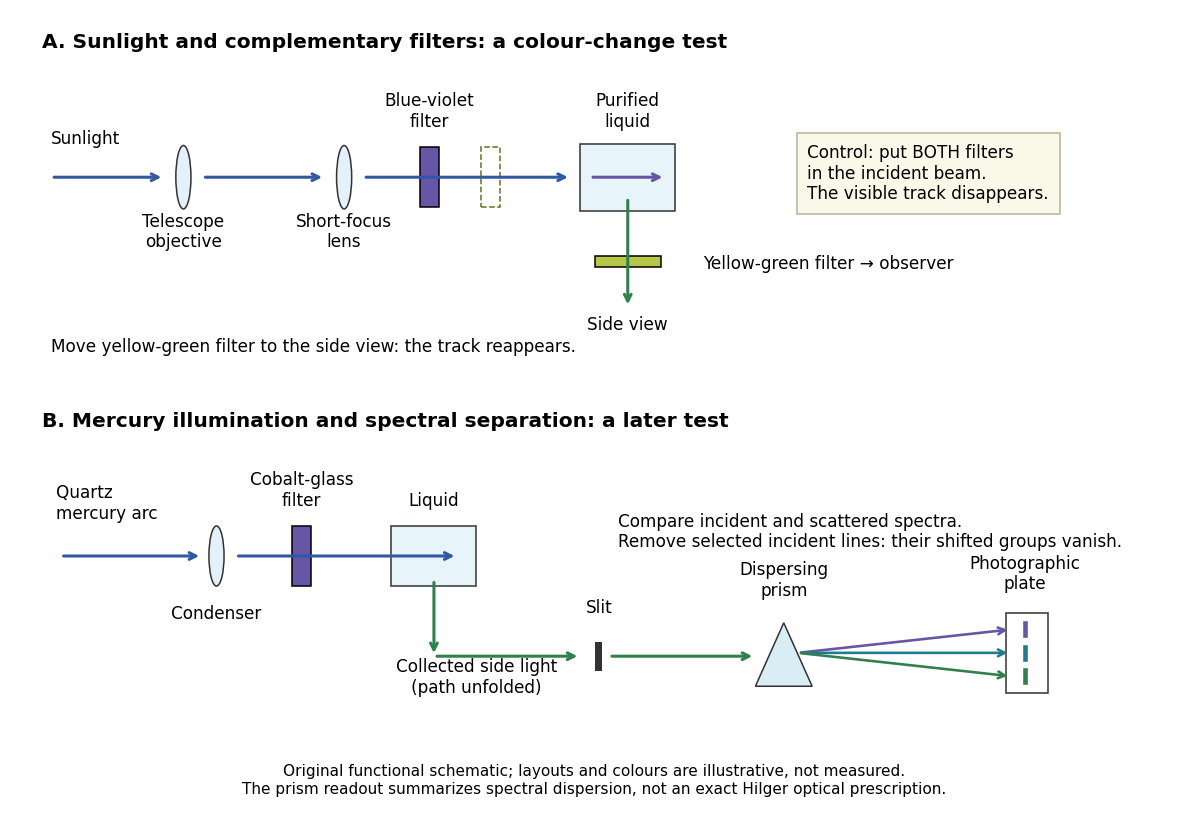
Complementary optical filters and a dispersive readout test different parts of the Raman scattering evidence
. Original functional schematic of the filter test and later spectral test. Side collection is unfolded for readability. The optical prism, spectrograph slit and photographic plate indicate dispersion and recording; the sketch supplies no historical distances, exact optical prescription or measured colour intensities. Source. Details.
Their May 1928 report strengthens the comparison: filtered mercury illumination of toluene produced extra spectral lines. Removing the incident line removed its associated longer-wavelength group; a quinine filter removing the , and group removed a different shifted group while preserving the one associated with . These are actual selective-excitation controls, rather than inferred colours.[ref]
The Optical Analogue of the Compton Effect by Chandrasekhara Venkata Raman and Kariamanikkam Srinivasa Krishnan. Raman and Krishnan, The Optical Analogue of the Compton Effect, Nature 121, p. 711, Fig. 1 description and removal of individual incident-line groups
The inference has limits. A complementary-filter test alone establishes newly admitted wavelengths, not their precise spacing or a unique microscopic mechanism. Fluorescence can also survive purification when intrinsic to the liquid, and fluorescence can be polarized. Useful distinctions therefore combine resolved spectral lines, excitation dependence, wave polarization and sample preparation. A proposed modern extension is to change a single incident frequency: a molecular Raman shift should follow the same internal energy gap, whereas ordinary relaxed molecular fluorescence usually retains approximately its emission-band positions. This is a diagnostic under stated conditions, not a universal theorem about every fluorescent material or resonant scattering process. Raman scattering need not involve a populated, relaxed electronic excited state as ordinary molecular fluorescence does; neither a redder photon nor the word Stokes identifies the mechanism by itself.
The 1930 Nobel Prize in Physics went to Chandrasekhara Venkata Raman alone for his work on scattering of light and the discovery of the effect. That award allocation should be distinguished from the joint experimental report with Kariamanikkam Srinivasa Krishnan.[ref]
The Nobel Prize in Physics 1930 by Nobel Foundation. Nobel Foundation prize record: sole laureate and award motivation, Physics 1930
Two-load radiometer calibration 2026-10-18
For a stable radiometer with affine output , let be the fixed response coefficient and the receiver noise temperature. Two reference loads with known equivalent input noise temperatures give outputs and . Subtracting their outputs eliminates ; dividing source and reference differences eliminates :This two-load radiometer calibration assumes unchanged response and receiver noise temperature between readings, with the loads and source referred to the same input. It also eliminates an additional constant output offset. Physical load temperatures must first be converted to the applicable equivalent input noise temperatures when the classical thermal approximation fails. The Penzias-Wilson microwave background experiment gives an original worked example.
Noise temperature Created 2026-10-18 Updated 2026-10-25
A noise temperature expresses received or internally added noise power on an equivalent temperature scale. For one matched receiving channel in the classical thermal limit, an ideal rectangular bandwidth gives , with Boltzmann constant . An equivalent noise temperature need not equal a component's physical temperature.
Radiocarbon calibration 2026-10-18
Radiocarbon calibration converts conventional radiocarbon ages into calendar-age information using independently dated material and models of changes in reservoir isotope ratios. Conventional ages use the historical -year half-life, whereas the physical carbon-14 half-life is about years.[ref]
Radiocarbon calibration by Oxford Radiocarbon Accelerator Unit. Half-life conventions, changing atmospheric ratios and tree-ring calibration
Radiocarbon age 2026-10-18
A radiocarbon age estimates elapsed time from a measured carbon-14 ratio , an assumed initial ratio and a specified nuclear decay constant . The displayed exponential decay inversion gives the age on that model's timescale. A conventional radiocarbon age uses a prescribed reference and decay convention; it is not generally a calendar age. Radiocarbon calibration accounts for changes in the atmospheric isotope ratio and maps the measurement to a calendar-age estimate.
There are unlisted articles, also show them or only show them.