
Inverse-function linearization of a first-order equation Created 2026-10-18 Updated 2026-10-20
On a branch where a differentiable function has a nonzero derivative, the inverse function theorem allows the ordinary differential equation to be rewritten for . A nonlinear equation in one direction can become a linear ordinary differential equation in the other. For example, becomesThe integrating factor gives , hence . This family must retain the original denominator restriction . The separate zero solution on intervals avoiding is lost by the inversion and must be restored.
Failure probabilities for two independent lifetimes Created 2026-10-18 Updated 2026-11-05
For independent survival times with cumulative distribution functions , the probability both components have failed by time isThe probability at least one has failed isThe first equality uses independence of random variables; the second applies it to the complementary event that both survive. These are the distributions of the two extreme order statistics.
Marginal distributions alone do not determine these probabilities. Without independence, the Fréchet inequalities give , and inclusion-exclusion gives .
Conjugation preserves element order Created 2026-10-18 Updated 2026-11-05
For every positive integer , cancellation gives . Thus the power on one side is the identity element exactly when , proving preservation of the order of a group element, including infinite order. In particular, and are conjugate because , and hence have the same order.
An element and its inverse have the same order Created 2026-10-18 Updated 2026-11-05
For every positive integer , , hence if and only if . The sets of positive powers returning to the identity element are therefore equal. Taking the least positive exponent therefore gives the same finite order of a group element for and ; if the sets are empty, both elements have infinite order. Equivalently, and generate the same cyclic subgroup.
Transform-limited pulse 2026-10-18
An optical pulse with constant group delay over its spectrum. At fixed spectral amplitude, its power-weighted temporal variance is minimal.
Pulse compression 2026-10-18
Intensity autocorrelation 2026-10-18
A diagnostic proportional to for delay . It does not uniquely reconstruct a complex optical electric field; extracting pulse duration requires a shape model.
Time-bandwidth product Created 2026-10-18 Updated 2026-10-20
The product of a specified temporal width and spectral frequency width. State whether each width refers to power or field amplitude and whether it is a full width at half maximum or a standard deviation.
Dark-field microscopy Created 2026-10-18 Updated 2026-11-05
Dark-field microscopy excludes directly transmitted illumination from the microscope objective, while admitting light scattered by the specimen. A transparent particle can then appear bright against a dark background even when it has little optical absorption.
One implementation illuminates the specimen with a hollow cone whose direct rays pass outside the objective's acceptance cone. Scattering of light at particles or edges redirects some of this illumination into the objective. Dust and scratches also become bright, so a clean blank specimen is a useful control.[ref]
Darkfield Illumination by Nikon Instruments Inc.. Illumination geometry and discussion of light scattered into the objective
Detection is not the same as optical resolution: a very small particle may be visible as an unresolved spot whose width is set by the point spread function.
Bright-field microscopy 2026-10-18
Transmitted-light imaging with an optical microscope in which the directly transmitted illumination contributes the bright background. An absorbing specimen can reduce that background locally. The ideal lossless phase object calculation in coherent zero-mode model of phase contrast shows why ordinary brightness detection need not reveal every optical variation.
Rayleigh optical gradient force 2026-10-18
The geometrical optics account of an optical trap adds the momentum flux changes of refracted and reflected light rays. It applies when the bead is large compared with the surrounding medium's wavelength. When the bead is much smaller, an induced electric dipole gives a different approximation. For a homogeneous dielectric sphere of radius , define , with the peak complex electric field and its SI polarizability. In a transparent, nonmagnetic, nondispersive host,where are particle and host refractive indices, is cycle-averaged light intensity, is the vacuum permittivity and is the speed of light. The quasistatic electric dipole approximation requires , with the vacuum wavelength, and a field nearly uniform across the bead.
For real quasistatic , building an induced electric dipole gives instantaneous potential energy . Averaging over one optical cycle givesThus gives positive polarizability and attraction toward larger light intensity; reverses this contribution. The factor uses a peak field: substituting a root mean square field without changing that factor would halve the force incorrectly. Dimensionally is energy, so its gradient is force.
This leading conservative term does not remove the optical scattering force. Even a nonabsorbing induced electric dipole reradiates light: at fixed wavelength and index contrast, its Rayleigh scattering cross-section scales as , while scales as . A smaller bead can therefore improve the ratio of gradient to scattering forces while weakening the well relative to , where is the Boltzmann constant and the temperature. Optical force balance and resistance to thermal escape are separate questions. Intermediate bead sizes require a wave-scattering calculation; neither a ray calculation nor this small-dipole expression is uniformly valid there.
Gain bandwidth Created 2026-10-18 Updated 2026-10-25
The frequency range over which an amplifying medium supplies appreciable optical gain. Its width must be stated with a gain-profile convention.
Optical frequency measurement with a comb 2026-10-18
Mix an unknown single-frequency laser with a nearby comb tooth on a photodiode. Define the signed beat , soThe beat arises from the cross term in light intensity:An electronic detector can follow this slow difference even though it cannot resolve either optical oscillation. The square-law expression also shows why a real-valued intensity trace by itself loses the sign of . A small known upward shift of the chosen tooth decreases when the unknown lies above it and increases when it lies below, provided the tooth assignment remains unchanged.
For an original example, stipulateThen and . Choosing the opposite sign would give instead. The stipulated optical frequency is countable because the large optical value is expressed using the integer and three electronic frequencies; the diagram's two controls establish the comb, and this additional beat places the unknown against it.
Comb self-referencing 2026-10-18
Comb self-referencing compares two parts of one optical frequency comb. Coherent broadening supplies an octave, a factor of two in frequency. Second-harmonic generation doubles a red tooth; a photodiode detects its beat with an original blue tooth.[ref]
Introduction to Self-reference Comb Laser by Comblaser Laboratory, Department of Physics, National Central University. Introduction to Self-reference Comb Laser, Fig.1 explanation
Applying the tooth formula givesThe doubled branch carries , while the original high-frequency branch carries : their difference retains exactly one offset.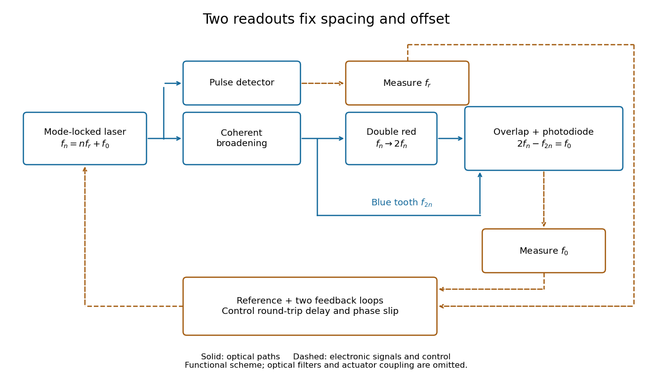
Read the tooth spacing and offset through separate electronic signals
. Original functional comb self-referencing scheme. Solid optical paths bring doubled red light and original blue light to one detector. Dashed electronic paths connect both readouts to a common reference and feedback controls. Actuators can affect both parameters. Details.
The displayed difference uses the order doubled tooth minus original tooth. An ordinary electronic frequency counter returns a nonnegative beat magnitude; spectral selection and known electronic shifts must identify whether it represents , , or a shifted version. Coherent broadening, overlapping photon polarization, spatial alignment and temporal overlap are required. Merely producing a broad patch of colored light does not establish a usable offset signal.
Carrier-envelope offset frequency 2026-10-18
The carrier-envelope offset frequency expresses the carrier's pulse-to-pulse phase slip relative to its envelope. Fixing the repetition frequency leaves this slip undetermined.[ref]
Defining and Measuring Optical Frequencies: The Optical Clock Opportunity – and More by John L. Hall. Defining and Measuring Optical Frequencies: The Optical Clock Opportunity – and More, p.131: offset
With the positive-exponential convention derived above, modulo . Changing translates every tooth equally; differentiating at fixed givesThus at , a chosen change in spacing moves that tooth by if stays fixed. The large multiplier is why a stable-looking pulse train is insufficient for accurate optical metrology. Mode locking 2026-10-18
Mode locking fixes relative phases between longitudinal normal modes of a laser, allowing short optical pulses. The same optical spectrum with wandering relative phases would not supply that stable pulse train.[ref]
Passion for Precision by Theodor W. Hänsch. Passion for Precision, p.157: coupled modes
Here is an original finite-mode model, with the convention that a positive frequency has time dependence :These field coefficients follow a Gaussian function and have aligned phases at . Choose and write . Since for every integer ,The pulse light intensity repeats every although the field needs four periods to repeat. At the pulse centers, , , and . A detector of light intensity alone therefore cannot distinguish this offset from zero. This model has far fewer teeth than a practical optical comb; its normalized time and frequency scales are chosen to make the carrier oscillations visible.
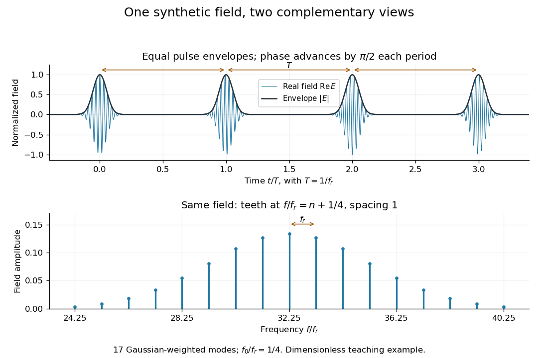

A short proof of the converse uses the Fourier series. If , then is periodic with period . Its Fourier series has frequencies ; restoring the removed factor shifts every tooth by . A finite observation time broadens the spectral peaks; it does not change this ideal infinite-train relation.
Guiding light and retaining useful optical power are different achievements. Charles Kuen Kao and George Alfred Hockham argued that impurities need not impose the measured losses of existing glasses on every future optical fiber. Their 1966 paper treats wave absorption, scattering of light and guidance separately; reducing impurity absorption leaves intrinsic material losses and geometric losses to address. This was a route toward practical communication, building on existing optical fibers, rather than the invention of every use of guided light.[ref]
Dielectric-fibre surface waveguides for optical frequencies by Charles Kuen Kao and George Alfred Hockham. pp. 1152–1154, §§3.1–4.2; p. 1158, §7
The launch experiment used clad glass optical fibers fixed in capillary tubes with epoxy for end polishing. Laser illumination gave transverse normal mode patterns; input-spot displacement and polarization of an electromagnetic wave controlled excitation. These observations tested guidance, not kilometre-scale optical fiber attenuation.[ref]
Dielectric-fibre surface waveguides for optical frequencies by Charles Kuen Kao and George Alfred Hockham. pp. 1157–1158, §6.2, Fig. 15, Table 2
Charles Kuen Kao's lecture describes the complementary material experiment: short, polished glass samples, including plasma-deposited fused silicon dioxide, were examined with purpose-built single-beam and later double-beam spectrophotometers. A separate ellipsometry measurement assessed end-surface specular reflection, a check against confusing interface loss with bulk wave absorption. The readout was loss versus wavelength. Comparing glass samples supported impurity reduction as a route to lower loss. Surface contamination and the tiny bulk loss of short samples limited inference; the result did not itself demonstrate a long drawn optical fiber. The lecture also credits subsequent manufacturing work at Corning.[ref]
Nobel Lecture: Sand from centuries past: Send future voices fast by Charles Kuen Kao. Published 2010 version of the 2009 lecture, p. 2302, §V, short-sample measurements, ellipsometer and later fiber manufacture
An original scale comparison makes the material problem tangible. In the uniform optical fiber attenuation model, a stipulated leaves of launched optical power after ; a stipulated leaves . Both guides could satisfy the same total internal reflection condition. A successful spot pattern at the output therefore cannot by itself establish a useful communication distance.
Fiber Bragg grating Created 2026-10-18 Updated 2026-11-05
A fiber Bragg grating is a longitudinally periodic refractive index modulation in an optical fiber. Reflections from successive periods reinforce near the vacuum wavelength , where is the period and is the guided mode's effective refractive index.
It acts as a wavelength-selective reflector while much off-resonant light continues through the optical fiber. Stretching the fiber changes the period and usually the effective refractive index, moving the reflected peak. This supports strain sensing; temperature also shifts the peak, so a strain measurement needs temperature control or independent compensation.
Lorentz invariance of optical cavity resonance Created 2026-10-18 Updated 2026-10-25
A Lorentz transformation of a resonant optical cavity transforms both the electromagnetic field and the mirror worldlines. Boundary conditions and event-by-event phase matching remain satisfied. For a longitudinal boost, a cavity of rest length has length and unequal forward/backward frequencies . The coordinate round-trip time is , while the phase rate on a moving mirror is , so the round-trip phase is still . A stationary-mirror resonance formula with only length contraction inserted describes the wrong boundary-value problem.
On the positive half-line, the Green function for with a zero Dirichlet boundary condition at the origin and decay at infinity isIt is continuous, has derivative jump , and is nonnegative. It is the negative of the Dirichlet half-line Green function for d2 minus 1; the sign of the leading differential term matters.
There are unlisted articles, also show them or only show them.